5 Ecological Production Units
Description: Ecological Production Units
Found in: State of the Ecosystem - Gulf of Maine & Georges Bank (2018+), State of the Ecosystem - Mid-Atlantic (2018+)
Indicator category: Extensive analysis, not yet published
Contributor(s): Robert Gamble
Data steward: NA
Point of contact: Robert Gamble, robert.gamble@noaa.gov
Public availability statement: Ecological production unit (EPU) shapefiles are available here.
5.1 Methods
To define ecological production units (EPUs), we assembled a set of physiographic, oceanographic and biotic variables on the Northeast U.S. Continental Shelf, an area of approximately 264,000 km within the 200 m isobath. The physiographic and hydrographic variables selected have been extensively used in previous analyses of oceanic provinces and regions (e.g Roff and Taylor 2000). Primary production estimates have also been widely employed for this purpose in conjunction with physical variables (Longhurst 2007) to define ecological provinces throughout the world ocean.
We did not include information on zooplankton, benthic invertebrates, fish, protected species, or fishing patterns in our analysis. The biomass and production of the higher trophic level groups in this region has been sharply perturbed by fishing and other anthropogenic influences. Similarly, fishing patterns are affected by regulatory change, market and economic factors and other external influences.
Because these malleable patterns of change are often unconnected with underlying productivity, we excluded factors directly related to fishing practices. The physiographic variables considered in this analysis are listed in Table 5.1. They include bathymetry and surficial sediments. The physical oceanographic and hydrographic measurements include sea surface temperature, annual temperature span, and temperature gradient water derived from satellite observations for the period 1998 to 2007.
5.2 Adaptations for the State of the ecosystem report
The definition of an EPU, for all indices used in the State of the ecosystem report is as follows:
- For commercial data - EPUs are defined by Greater Atlantic Region Statistical Areas. See Commercial landings data
- For survey data - EPUs are defined by survey data
5.2.1 Data sources
Shipboard observations for surface and bottom water temperature and salinity in surveys conducted in spring and fall. Daily sea surface temperature (SST, °C) measurements at 4 km resolution were derived from nighttime scenes composited from the AVHRR sensor on NOAA’s polar-orbiting satellites and from NASA’s MODIS TERRA and MODIS AQUA sensors. We extracted information for the annual mean SST, temperature span, and temperature gradients from these sources. The latter metric provides information on frontal zone locations.
| Variables | Sampling Method | Units |
|---|---|---|
| Surficial Sediments | Benthic Grab | Krumbian Scale |
| Sea Surface Temperature | Satellite Imagery (4km grid) | °C annual average |
| Sea Surface Temperature | Satellite Imagery (4km grid) | dimensionless |
| Sea Surface Temperature | Satellite Imagery (4km grid) | °C annual average |
| Surface Temperature | Shipboard hydrography (point) | °C (Spring and Fall) |
| Bottom Temperature | Shipboard hydrography (point) | °C (Spring and Fall) |
| Surface Salinity | Shipboard hydrography (point) | psu (Spring and Fall) |
| Bottom Salinity | Shipboard hydrography (point) | psu (Spring and Fall) |
| Stratification | Shipboard hydrography (point) | Sigma-t units (Spring and Fall) |
| Chlorophyll-a | Satellite Imagery (1.25 km grid) | mg/C/m3 (annual average) |
| Chlorophyll-a gradient | Satellite Imagery (1.25 km grid) | dimensionless |
| Chlorophyll-a span | Satellite Imagery (1.25 km grid) | mg/C/m3 (annual average) |
| Primary Production | Satellite Imagery (1.25 km grid) | gC/m3/year (cumulative) |
| Primary Production gradient | Satellite Imagery (1.25 km grid) | dimensionless |
| Primary Production span | Satellite Imagery (1.25 km grid) | gC/m3/year (cumulative) |
The biotic measurements included satellite-derived estimates of chlorophyll a (CHLa) mean concentration, annual span, and CHLa gradients and related measures of primary production. Daily merged SeaWiFS/MODIS-Aqua CHLa (CHL, mg m-3) and SeaiWiFS photosynthetically available radiation (PAR, Einsteins m-2 d-1) scenes at 1.25 km resolution were obtained from NASA Ocean Biology Processing Group.
5.2.3 Data analysis
In all cases, we standardized the data to common spatial units by taking annual means of each observation type within spatial units of 10’ latitude by 10’ longitude to account for the disparate spatial and temporal scales at which these observations are taken. There are over 1000 spatial cells in this analysis. Shipboard sampling used to obtain direct hydrographic measurements is constrained by a minimum sampling depth of 27 m specified on the basis of prescribed safe operating procedures. As a result nearshore waters are not fully represented in our initial specifications of ecological production units.
The size of the spatial units employed further reflects a compromise between retaining spatial detail and minimizing the need for spatial interpolation of some data sets. For shipboard data sets characterized by relatively coarse spatial resolution, where necessary, we first constructed an interpolated map using an inverse distance weighting function before including it in the analysis. Although alternative interpolation schemes based on geostatistical approaches are possible, we considered the inverse distance weighting function to be both tractable and robust for this application.
We first employed a spatial principal components analysis [PCA; e.g. Pielou (1984); Legendre and Legendre (1998)] to examine the multivariate structure of the data and to account for any inter-correlations among the variables to be used in subsequent analysis. The variables included in the analysis exhibited generally skewed distributions and we therefore transformed each to natural logarithms prior to analysis.
The PCA was performed on the correlation matrix of the transformed observations. We selected the eigenvectors associated with eigenvalues of the dispersion matrix with scores greater than 1.0 [the Kaiser-Guttman criterion; Legendre and Legendre (1998)] for all subsequent analysis. These eigenvectors represent orthogonal linear combinations of the original variables used in the analysis.
We delineated ecological subunits by applying a disjoint cluster based on Euclidean distances using the K-means procedure (Legendre and Legendre 1998) on the principal component scores The use of non-independent variables can strongly influence the results of classification analyses of this type (Pielou 1984), hence the interest in using the PCA results in the cluster.
The eigenvectors were represented as standard normal deviates. We used a Pseudo-F Statistic described by Milligan and Cooper (1985) to objectively define the number of clusters to use in the analysis. The general approach employed is similar to that of Host et al. (1996) for the development of regional ecosystem classifications for terrestrial systems.
After the analyses were done, we next considered options for interpolation of nearshore boundaries resulting from depth-related constraints on shipboard observations. For this, we relied on information from satellite imagery. For the missing nearshore areas in the Gulf of Maine and Mid-Atlantic Bight, the satellite information for chlorophyll concentration and sea surface temperature indicated a direct extension from adjacent observations. For the Nantucket Shoals region south of Cape Cod, similarities in tidal mixing patterns reflected in chlorophyll and temperature observations indicated an affinity with Georges Bank and the boundaries were changed accordingly.
Finally, we next considered consolidation of ecological subareas so that nearshore regions are considered to be special zones nested within the adjacent shelf regions. Similar consideration led to nesting the continental slope regions within adjacent shelf regions in the Mid-Atlantic and Georges Bank regions. This led to four major units: Mid-Atlantic Bight, Georges Bank, Western-Central Gulf of Maine (simply “Gulf of Maine” in the State of the Ecosystem), and Scotian Shelf-Eastern Gulf of Maine. As the State of the Ecosystem reports are specific to FMC managed regions, the Scotian Shelf-Eastern Gulf of Maine EPU is not considered in SOE indicator analyses.
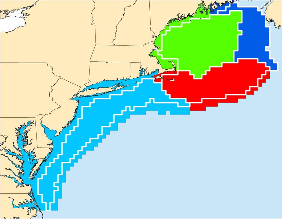
Figure 5.1: Map of the four Ecological Production Units, including the Mid-Atlantic Bight (light blue), Georges Bank (red), Western-Central Gulf of Maine (or Gulf of Maine; green), and Scotian Shelf-Eastern Gulf of Maine (dark blue)