Generating Simulated Data

Simulating input data from an ecosystem model

Here we use existing Atlantis ecosystem model output to generate input datasets for a variety of simpler population models, so that the performance of these models can be evaluated against known (simulated) ecosystem dynamics. Atlantis is an end-to-end spatial ecosystem model capable of including climate effects, seasonal migration, food web, and fishery interactions (Audzijonyte et al., 2019).

We extract simulated data using the R package atlantisom. The purpose of atlantisom is to use existing Atlantis model output to generate input datasets for a variety of models, so that the performance of these models can be evaluated against known (simulated) ecosystem dynamics. The process is briefly described here. Atlantis models can be run using different climate forcing, fishing, and other scenarios. Users of atlantisom specify fishery independent and fishery dependent sampling in space and time, as well as species-specific catchability, selectivty, and other observation processes for any Atlantis scenario. Internally consistent multispecies and ecosystem datasets with known observation error characteristics are atlantisom outputs, for use in individual model performance testing, comparing performance of alternative models, and performance testing of model ensembles against “true” Atlantis outputs.

The simulated dataset is based on output of the Norwegian and Barents Sea (NOBA) Atlantis model (Hansen et al., 2016, 2019). The simulated dataset contains comparable survey, fishery, and composition data as the Georges Bank dataset, but the time series span 80 simulation years and include 11 species. This dataset was used for initial model development, code quality testing, and model skill assessment by the modeling teams. Details of the dataset including construction and basic attributes are below.

Species in the ms-keyrun dataset

Our initial species selection includes 11 single species groups from the Atlantis NOBA model.

Generate the species table

lname <- data.frame(Name= c("Long_rough_dab",
                                 "Green_halibut",
                                 "Mackerel",
                                 "Haddock",
                                 "Saithe",
                                 "Redfish",
                                 "Blue_whiting",
                                 "Norwegian_ssh",
                                 "North_atl_cod",
                                 "Polar_cod",
                                 "Capelin"),
                    Long.Name = c("Long rough dab",
                                 "Greenland halibut",
                                 "Mackerel",
                                 "Haddock",
                                 "Saithe",
                                 "Redfish",
                                 "Blue whiting",
                                 "Norwegian spring spawning herring",
                                 "Northeast Atlantic Cod",
                                 "Polar cod",
                                 "Capelin"),
                    Latin = c("*Hippoglossoides platessoides*",
                              "*Reinhardtius hippoglossoides*",
                              "*Scomber scombrus*",
                              "*Melongrammus aeglefinus*",
                              "*Pollachius virens*",
                              "*Sebastes mentella*",
                              "*Micromesistius poutassou*",
                              "*Clupea harengus*",
                              "*Gadus morhua*",
                              "*Boreogadus saida*",
                              "*Mallotus villosus*"),
                    Code = c("LRD", "GRH", "MAC", "HAD", "SAI", "RED", 
                             "BWH", "SSH", "NCO", "PCO", "CAP")
)

# sppsubset <- merge(fgs, lname, all.y = TRUE)
# spptable <- sppsubset %>% 
#   arrange(Index) %>%
#   select(Name, Long.Name, Latin)

spptable <- lname %>%
   select(Name, Long.Name, Latin)

Model name	Full name	Latin name
Long_rough_dab	Long rough dab	Hippoglossoides platessoides
Green_halibut	Greenland halibut	Reinhardtius hippoglossoides
Mackerel	Mackerel	Scomber scombrus
Haddock	Haddock	Melongrammus aeglefinus
Saithe	Saithe	Pollachius virens
Redfish	Redfish	Sebastes mentella
Blue_whiting	Blue whiting	Micromesistius poutassou
Norwegian_ssh	Norwegian spring spawning herring	Clupea harengus
North_atl_cod	Northeast Atlantic Cod	Gadus morhua
Polar_cod	Polar cod	Boreogadus saida
Capelin	Capelin	Mallotus villosus

Generating a dataset

Configuration files specified once

NOBA_sacc38Config.R specifies location and names of files needed for atlantisom to initialize:

d.name <- here("simulated-data/atlantisoutput","NOBA_sacc_38")
functional.groups.file <- "nordic_groups_v04.csv"
biomass.pools.file <- "nordic_biol_v23.nc"
biol.prm.file <- "nordic_biol_incl_harv_v_011_1skg.prm"
box.file <- "Nordic02.bgm"
initial.conditions.file <- "nordic_biol_v23.nc"
run.prm.file <- "nordic_run_v01.xml"
scenario.name <- "nordic_runresults_01"
bioind.file <- "nordic_runresults_01BiomIndx.txt"
catch.file <- "nordic_runresults_01Catch.txt"
annage <- TRUE
fisheries.file <- "NoBAFisheries.csv"

omdimensions.R standardizes timesteps, etc. (this is part of atlantisom and should not need to be changed by the user):

#survey species inherited from omlist_ss
survspp <- omlist_ss$species_ss
# survey season and other time dimensioning parameters
# generalized timesteps all models
noutsteps <- omlist_ss$runpar$tstop/omlist_ss$runpar$outputstep
timeall <- c(0:noutsteps)
stepperyr <- if(omlist_ss$runpar$outputstepunit=="days") 365/omlist_ss$runpar$toutinc
midptyr <- round(median(seq(0,stepperyr)))

# model areas, subset in surveyconfig
allboxes <- c(0:(omlist_ss$boxpars$nbox - 1))

# fishery output: learned the hard way this can be different from ecosystem outputs
fstepperyr <- if(omlist_ss$runpar$outputstepunit=="days") 365/omlist_ss$runpar$toutfinc

# survey selectivity (agecl based)
sp_age <- omlist_ss$funct.group_ss[, c("Name", "NumCohorts", "NumAgeClassSize")]

# should return all age classes fully sampled (Atlantis output is 10 age groups per spp)
n_age_classes <- sp_age$NumCohorts
# changed below for multiple species NOTE survspp alphabetical; NOT in order of fgs!!
# this gives correct names
age_classes <- lapply(n_age_classes, seq)
names(age_classes)<-sp_age$Name

n_annages <- sp_age$NumCohorts * sp_age$NumAgeClassSize
# changed below for multiple species
annages <- lapply(n_annages, seq)
names(annages)<-sp_age$Name

Change these survey and fishery config files

mssurvey_spring.R and mssurvey_fall.R configure the fishery independent surveys (in this census test, surveys sample all model polygons in all years and have efficiency of 1 for all species, with no size selectivity):

# Default survey configuration here has a range of efficiencies and selectivities
# To emulate a range of species in a single multispecies survey
# Also now happens in "spring" and "fall"
# Need to define survey season, area, efficiency, selectivity

# Survey name
survey.name="BTS_spring_allbox_effic1"

#Atlantis model timestep corresponding to the true output--now from census_spec.R
timestep <- stepperyr #5

#Which atlantis timestep does the survey run in?--now from census_spec.R
# with 5 output steps per year, 0 is Jan-Feb-midMar, 1 is midMar-Apr-May, 
# 2 is June-July-midAug, 3 is midAug-Sept-Oct, 4 is Nov-Dec (ish)

# No, timestep 0 is initial condition and should be ignored to align 
# snapshots (biomass, numbers) with
# cumulative outputs (fishery catch, numbers)

# with 5 output steps per (non leap) year:
# 1 is day 73, or 14 March
# 2 is day 146, or 26 May
# 3 is day 219, or 7 August
# 4 is day 292, or 19 October
# 5 is day 365, or 31 December

survey_sample_time <- 1 # spring survey

#The last timestep to sample
total_sample <- noutsteps-1 #495

#Vector of indices of survey times to pull
survey_sample_full <- seq(survey_sample_time,
                          total_sample, by=timestep)

survtime <- survey_sample_full

# survey area
# should return all model areas
survboxes <- allboxes

# survey efficiency (q)
# should return a perfectly efficient survey 
surveffic <- data.frame(species=survspp,
                     efficiency=rep(1.0,length(survspp)))

# survey selectivity (agecl based)
# this is by age class, need to change to use with ANNAGEBIO output
#survselex <- data.frame(species=rep(names(age_classes), each=n_age_classes),
#                     agecl=rep(c(1:n_age_classes),length(survspp)),
#                     selex=rep(1.0,length(survspp)*n_age_classes))

# for annage output uses names(annages) NOT alphabetical survspp
survselex <- data.frame(species=rep(names(annages), n_annages), #  
                        agecl=unlist(sapply(n_annages,seq)),
                        selex=rep(1.0,sum(n_annages)))

survselex.agecl <- survselex


# effective sample size needed for sample_fish
# this effective N is high but not equal to total for numerous groups
surveffN <- data.frame(species=survspp, effN=rep(100000, length(survspp)))

# survey index cv needed for sample_survey_xxx
# cv = 0.1
surv_cv <- data.frame(species=survspp, cv=rep(0.1,length(survspp)))

# length at age cv for input into calc_age2length function
# function designed to take one cv for all species, need to change to pass it a vector
lenage_cv <- 0.1

# max size bin for length estimation, function defaults to 150 cm if not supplied
maxbin <- 200

# diet sampling parameters
alphamult <- 10000000
unidprey <- 0

# Default survey configuration here has a range of efficiencies and selectivities
# To emulate a range of species in a single multispecies survey
# Also now happens in "spring" and "fall"
# Need to define survey season, area, efficiency, selectivity

# Survey name
survey.name="BTS_fall_allbox_effic1"

#Atlantis model timestep corresponding to the true output--now from census_spec.R
timestep <- stepperyr #5

#Which atlantis timestep does the survey run in?--now from census_spec.R
# with 5 output steps per year, 0 is Jan-Feb-midMar, 1 is midMar-Apr-May, 
# 2 is June-July-midAug, 3 is midAug-Sept-Oct, 4 is Nov-Dec (ish)

# No, timestep 0 is initial condition and should be ignored to align 
# snapshots (biomass, numbers) with
# cumulative outputs (fishery catch, numbers)

# with 5 output steps per (non leap) year:
# 1 is day 73, or 14 March
# 2 is day 146, or 26 May
# 3 is day 219, or 7 August
# 4 is day 292, or 19 October
# 5 is day 365, or 31 December

survey_sample_time <- 3 # fall survey

#The last timestep to sample
total_sample <- noutsteps-1 #495

#Vector of indices of survey times to pull
survey_sample_full <- seq(survey_sample_time,
                          total_sample, by=timestep)

survtime <- survey_sample_full

# survey area
# should return all model areas
survboxes <- allboxes

# survey efficiency (q)
# should return a perfectly efficient survey 
surveffic <- data.frame(species=survspp,
                     efficiency=rep(1.0,length(survspp)))

# survey selectivity (agecl based)
# this is by age class, need to change to use with ANNAGEBIO output
#survselex <- data.frame(species=rep(survspp, each=n_age_classes),
#                     agecl=rep(c(1:n_age_classes),length(survspp)),
#                     selex=rep(1.0,length(survspp)*n_age_classes))

# for annage output
survselex <- data.frame(species=rep(names(annages), n_annages), #  
                        agecl=unlist(sapply(n_annages,seq)),
                        selex=rep(1.0,sum(n_annages)))

survselex.agecl <- survselex 


# effective sample size needed for sample_fish
# this effective N is high but not equal to total for numerous groups
surveffN <- data.frame(species=survspp, effN=rep(100000, length(survspp)))

# survey index cv needed for sample_survey_xxx
# cv = 0.1
surv_cv <- data.frame(species=survspp, cv=rep(0.1,length(survspp)))

# length at age cv for input into calc_age2length function
# function designed to take one cv for all species, need to change to pass it a vector
lenage_cv <- 0.1

# max size bin for length estimation, function defaults to 150 cm if not supplied
maxbin <- 200

# diet sampling parameters
alphamult <- 10000000
unidprey <- 0

msfishery.R configures the fishery dependent data:

# Default fishery configuration here is a census
# June 2023 now aggregating over fleets in input
# change name to identify fleet specific config files
# output will be stored with this name

fishery.name="allfleet"

# select fleets by number from fisheries.csv Index column
# NULL is all fleets
fishfleets <- NULL

# Inherits species from input omlist_ss
fishspp <- omlist_ss$code_ss 

# fishery output: learned the hard way this can be different from ecosystem outputs
fstepperyr <- if(omlist_ss$runpar$outputstepunit=="days") 365/omlist_ss$runpar$toutfinc

#The last timestep to sample
total_sample <- noutsteps-1 #495

# leave out model burn in period? define how long
burnin <- 0

# take only some years? for mskeyrun we do this later, here take all
nyears <- NULL

# same time dimensioning parameters as in surveycensus.R
#Vector of indices of catch in numbers to pull (by timestep to sum)
fish_sample_full <- c(0:total_sample)  #total_sample
#fish_burnin <- burnin*fstepperyr+1
#fish_nyears <- nyears*fstepperyr
#fish_times <- fish_sample_full[fish_burnin:(fish_burnin+fish_nyears-1)]
#fish_timesteps <- seq(fish_times[fstepperyr], max(fish_times), by=fstepperyr) #last timestep
#fish_years <- unique(floor(fish_times/fstepperyr)+1) # my original
#fish_years <- unique(floor(fish_times/fstepperyr)) #from Christine's new sardine_config.R

#fishtime <- fish_times

fishtime <- fish_sample_full

# fishery sampling area
# should return all model areas, this assumes you see everything that it caught
fishboxes <- c(0:(omlist_ss$boxpars$nbox - 1))

# effective sample size needed for sample_fish
# this effective N is divided by the number of annual timesteps below, so 200 per time
# use as input to the length samples, ages can be a subset
fisheffN <- data.frame(species=survspp, effN=rep(1000, length(survspp)))

#this adjusts for subannual fishery output so original effN is for whole year
fisheffN$effN <- fisheffN$effN/fstepperyr 

# fishery catch cv can be used in sample_survey_biomass
# perfect observation
fish_cv <- data.frame(species=fishspp, cv=rep(0.01,length(fishspp)))

Run atlantisom and save outputs

True datasets are generated as follows, using atlantisom wrapper functions om_init to assemble initial true atlantis data, om_species to subset true data for desired species, om_index to generate survey biomass and total catch biomass indices, om_comps to generate age and length compositions and average weight at age from surveys and fisheries, and om_diet to generate diet from surveys. Outputs are saved to the atlantisoutput folder (not kept on github due to size):

NOBAom <- om_init(here("data-raw/simulated-data/config/NOBA_sacc38Config.R"))

NOBAom_ms <- om_species(spptable$Name, NOBAom)

#need to change internal call to source in atlantisom om_index om_comps and om_diet functions
#expecting a config folder in same directory as rmd
#this is a workaround

dir.create(file.path(here("docs/config")))

file.copy(here("data-raw/simulated-data/config/omdimensions.R"), here("docs/config/omdimensions.R"))

NOBAom_ms_ind <- om_index(usersurvey = c(here("data-raw/simulated-data/config/mssurvey_spring.R"), 
                                         here("data-raw/simulated-data/config/mssurvey_fall.R")), 
                           userfishery = here("data-raw/simulated-data/config/msfishery.R"),
                           omlist_ss = NOBAom_ms, 
                           n_reps = 1, 
                           save = TRUE)

NOBAom_ms_comp <- om_comps(usersurvey = c(here("data-raw/simulated-data/config/mssurvey_spring.R"), 
                                         here("data-raw/simulated-data/config/mssurvey_fall.R")), 
                           userfishery = here("data-raw/simulated-data/config/msfishery.R"),
                           omlist_ss = NOBAom_ms, 
                           n_reps = 1, 
                           save = TRUE)

NOBAom_ms_diet <- om_diet(config = here("data-raw/simulated-data/config/NOBA_sacc38Config.R"),
                          dietfile = "NOBADetDiet.gz",
                          usersurvey = c(here("data-raw/simulated-data/config/mssurvey_spring.R"), 
                                         here("data-raw/simulated-data/config/mssurvey_fall.R")), 
                          omlist_ss = NOBAom_ms, 
                          n_reps = 1, 
                          save = TRUE)

unlink(here("docs/config"), recursive = TRUE)

Create mskeyrun simulated data

Scripts in ms-keyrun/data-raw show the process of making mskeyun datasets from atlantisom output generated above. Atlantis outputs and atlantisom outputs produced above are local to Sarah’s computer for this code to run, as they are too large for github. However, the scripts are linked here to show the process. Overall this script creates all datasets using functions specific to each data type:

Code to build simulated datasets

#' Sarah's notes for building simulated dataset
#' 
#' all atlantis files are local on my computer in folder
#' ms-keyrun/simlulated-data/atlantisoutput
#' 
#' see SimData.Rmd for how these are generated using atlantisom
#' 
#' to make data for package
#' source these files in data-raw/R:
#'
#' create_sim_focal_species.R
#' get_sim_survey_index.R
#' 
#' run from ms-keyrun directory

library(here)

atlmod <- here("data-raw/simulated-data/config/NOBA_sacc38Config.R")

create_sim_focal_species(atlmod)

create_sim_biolpar(atlmod)

create_sim_survey_info(atlmod)

create_sim_survey_index(atlmod, fitstart=40, fitend=120)

create_sim_fishery_index(atlmod, fitstart=40, fitend=120) #creates subannual amd aggregate

create_sim_survey_agecomp(atlmod, fitstart=40, fitend=120)

create_sim_fishery_agecomp(atlmod, fitstart=40, fitend=120)

create_sim_fishery_agecomp_subannual(atlmod, fitstart=40, fitend=120)

create_sim_survey_lencomp(atlmod, fitstart=40, fitend=120)

create_sim_fishery_lencomp(atlmod, fitstart=40, fitend=120)

create_sim_fishery_lencomp_subannual(atlmod, fitstart=40, fitend=120)

create_sim_survey_dietcomp(atlmod, fitstart=40, fitend=120)

create_sim_survey_bottemp(atlmod, fitstart=40, fitend=120)

create_sim_fishery_wtage(atlmod, fitstart=40, fitend=120)

create_sim_fishery_wtage_subannual(atlmod, fitstart=40, fitend=120)

create_sim_survey_wtage(atlmod, fitstart=40, fitend=120)

create_sim_survey_agelen(atlmod, fitstart=40, fitend=120)

create_sim_fishery_agelen(atlmod, fitstart=40, fitend=120)

create_sim_percapconsumption(atlmod, fitstart=40, fitend=120)

create_sim_startpars(atlmod, fitstart=40, fitend=120)

# food web model specific datasets add other species

create_sim_survey_index_fw(atlmod, fitstart=40, fitend=120)

create_sim_fishery_index_fw(atlmod, fitstart=40, fitend=120)

create_sim_survey_dietcomp_fw(atlmod, fitstart=40, fitend=120)

# below combines already loaded mskeyrun datasets,  
# outputs of create_sim_survey_agelen and create_sim_survey_dietcomp
# ensure that these are up to date before running

create_sim_survey_lendietcomp()

For example, create_sim_survey_index() takes the saved atlantisom output plus user specifications for fit start and end years to produce the dataset mskeyrun::simSurveyIndex:

#' Read in survey data save as rda
#' 
#' atlantosom output is accessed and surveys pulled over time
#' 
#'@param atlmod configuration file specifying Atlantis simulation model filenames 
#'and locations  
#'@param saveToData Boolean. Export to data folder (Default = T)
#'
#'@return A tibble (Also written to \code{data} folder)
#'\item{ModSim}{Atlantis model name and simulation id}
#'\item{year}{year simulated survey conducted}
#'\item{Code}{Atlantis model three letter code for functional group}
#'\item{Name}{Atlantis model common name for functional group}
#'\item{survey}{simulated survey name}
#'\item{variable}{biomass or coefficient of variation (cv) of biomass}
#'\item{value}{value of the variable}
#'\item{units}{units of the variable}
#'

library(magrittr)

create_sim_survey_index <- function(atlmod,fitstart=NULL,fitend=NULL,saveToData=T) {

  # input is path to model config file for atlantisom
  source(atlmod)
  
  # path for survey and fishery config files
  cfgpath <- stringr::str_extract(atlmod, ".*config")
  
  #works because atlantis directory named for model and simulation
  modpath <- stringr::str_split(d.name, "/", simplify = TRUE)
  modsim <- modpath[length(modpath)]
  
  #read in survey biomass data
  survObsBiom <- atlantisom::read_savedsurvs(d.name, 'survB') #reads in all surveys
  
  # get config files for survey cv
  svcon <- list.files(path=cfgpath, pattern = "*survey*", full.names = TRUE)
  
  # read true list with run and biol pars, etc
  omlist_ss <- readRDS(file.path(d.name, paste0(scenario.name, "omlist_ss.rds")))
  
  # model timesteps, etc from omdimensions script
  source(paste0(cfgpath,"/omdimensions.R"), local = TRUE)
  
  #Number of years
  nyears <- omlist_ss$runpar$nyears
  total_sample <- omlist_ss$runpar$tstop/omlist_ss$runpar$outputstep
  
  # user specified fit start and times if different from full run
  fitstartyr <- ifelse(!is.null(fitstart), fitstart-1, 0)
  fitendyr <- ifelse(!is.null(fitend), fitend, total_sample)
  
  atlantis_full <- c(1:total_sample)  
  mod_burnin <- fitstartyr*stepperyr+1
  fit_nyears <- fitendyr-fitstartyr
  fit_ntimes <- fit_nyears*stepperyr
  fittimes <- atlantis_full[mod_burnin:(mod_burnin+fit_ntimes-1)]
  #fit_timesteps <- seq(fittimes[stepperyr], max(fittimes), by=stepperyr) #last timestep
  #fit_years <- unique(floor(fittimes/stepperyr)) #from Christine's new sardine_config.R
  #fittimes.days <- if(omlist_ss$runpar$outputstepunit=="days") fittimes*omlist_ss$runpar$outputstep
  
  
  # survey cv lookup from config files
  svcvlook <- tibble::tibble()
  for(c in 1:length(svcon)){
    source(svcon[c], local = TRUE)
    surv_cv_n <- surv_cv %>% 
      dplyr::mutate(survey=survey.name)
    svcvlook <- dplyr::bind_rows(svcvlook, surv_cv_n)
  }
  
  allsvbio <- tibble::tibble()
  
  #multiple surveys named in list object
  for(s in names(survObsBiom)){
    #arrange into wide format: year, Species1, Species2 ... and write csv
    svbio <- survObsBiom[[s]][[1]] %>%
      dplyr::filter(time %in% fittimes) %>%
      dplyr::mutate(year = ceiling(time/stepperyr)) %>%
      dplyr::select(species, year, atoutput) %>%
      dplyr::rename(biomass = atoutput) %>%
      dplyr::left_join(dplyr::select(omlist_ss$funct.group_ss, Code, Name), by = c("species" = "Name")) %>%
      dplyr::mutate(ModSim = modsim) %>%
      dplyr::mutate(survey = s) %>%
      dplyr::left_join(svcvlook) %>%
      dplyr::select(ModSim, year, Code, Name=species, survey, everything()) %>%
      tidyr::pivot_longer(cols = c("biomass", "cv"), 
                          names_to = "variable",
                          values_to = "value") %>%
      dplyr::mutate(units = ifelse(variable=="biomass", "tons", "unitless")) %>%
      dplyr::arrange(Name, survey, variable, year)
    
    allsvbio <- dplyr::bind_rows(allsvbio, svbio)
  }
  
  simSurveyIndex <- allsvbio
  
  if (saveToData) {
    #saveRDS(focalSpecies,saveToRDS)
    usethis::use_data(simSurveyIndex, overwrite = TRUE)
  }
  
  return(simSurveyIndex)
  
  
}

All functions are in this mskeyrun repository folder: https://github.com/NOAA-EDAB/ms-keyrun/tree/master/data-raw/R

Additional simulated data for food web models

The data generated above focuses on the 11 fully age structured stocks. Here we add information needed for food web modeling on the remaining groups in the simulated system.

Code for remaining groups

# all NOBA species not already in mskeyrun dataset
fwspp <- atlantisom::load_fgs(here("data-raw/data"), "nordic_groups_v04.csv") %>% 
  dplyr::filter(IsTurnedOn == 1) %>%
  dplyr::select(Code, Name, Long.Name, isFished, InvertType) %>%
  dplyr::filter(!Name %in% spptable$Name)

Code	Name	Long.Name	isFished	InvertType
POB	Polar_bear	Polar Bear	0	MAMMAL
KWH	Killer_whale	Killer whale	0	MAMMAL
SWH	Sperm_whale	Sperm whale	0	MAMMAL
HWH	Humpb_whale	Humpback whale	0	MAMMAL
MWH	Minke_whale	Minke whale	1	MAMMAL
FWH	Fin_whale	Fin whale	0	MAMMAL
BES	Beard_seal	Bearded Seal	0	MAMMAL
HAS	Harp_seal	Harp Seal	0	MAMMAL
HOS	Hood_seal	Hooded Seal	0	MAMMAL
RIS	Ring_seal	Ringed Seal	0	MAMMAL
SBA	Sea_b_arct	Arctic seabirds	0	BIRD
SBB	Sea_b_bor	Boreal seabirds	0	BIRD
SHO	Sharks_other	Other sharks	0	SHARK
DEO	Demersals_other	Other demersals	1	FISH
PEL	Pelagic_large	Large pelagic fish	1	FISH
PES	Pelagic_small	Small pelagic fish	1	FISH
REO	Redfish_other	Other redfish	1	FISH
DEL	Demersal_large	Large demersals	1	FISH
FLA	Flatfish_other	Other flatfish	1	FISH
SSK	Skates_rays	Skates and rays	0	FISH
MES	Mesop_fish	Mesopelagic fish	1	FISH
PWN	Prawns	Prawns	1	PWN
CEP	Squid	Squid	0	CEP
KCR	King_crab	Red king crab	1	LG_INF
SCR	Snow_crab	Snow crab	1	FISH
ZG	Gel_zooplankton	Gelatinous zooplankton	0	LG_ZOO
ZL	Large_zooplankton	Large zooplankton	0	LG_ZOO
ZM	Medium_zooplankton	Medium zooplankton	0	MED_ZOO
ZS	Small_zooplankton	Small zooplankton	0	SM_ZOO
DF	Dinoflag	Dinoflagellates	0	DINOFLAG
PS	Small_phytop	Small phytoplankton	0	SM_PHY
PL	Large_phytop	Large phytoplankton	0	LG_PHY
BC	Predatory_ben	Predatory benthos	0	LG_INF
BD	Detrivore_ben	Detrivore benthos	0	LG_INF
BFF	Benthic_filterf	Benthic filter feeders	0	SED_EP_FF
SPO	Sponges	Sponges	0	SED_EP_FF
COR	Corals	Corals	0	SED_EP_FF
PB	Pel_bact	Pelagic bacteria	0	PL_BACT
BB	Ben_bact	Sediment bacteria	0	SED_BACT
DR	Ref_det	Refractory detritus	0	REF_DET
DL	Lab_det	Labile detritus	0	LAB_DET
DC	Carrion	Carrion	0	CARRION

This consists of survey biomass and diet, and fishery catch information for the non age-structured species.

To generate this, we apply selected functions from the atlantisom package with slightly modified config files to ensure the food web “fw” datasets don’t overwrite the multispecies datasets:

NOBAom <- om_init(here("data-raw/simulated-data/config/NOBA_sacc38Config.R"))

NOBAom_fw <- om_species(fwspp$Name, NOBAom, save = FALSE) #save by hand, don't overwrite 11 species omlist_ss

saveRDS(NOBAom_fw, file.path(d.name, paste0(scenario.name, "omlist_fw.rds")))

dir.create(file.path(here("vignettes/config")))

file.copy(here("data-raw/simulated-data/config/omdimensions.R"), here("vignettes/config/omdimensions.R"))

NOBAom_fw_ind <- om_index(usersurvey = c(here("data-raw/simulated-data/config/mssurvey_spring_fw.R"), 
                                         here("data-raw/simulated-data/config/mssurvey_fall_fw.R")), 
                           userfishery = here("data-raw/simulated-data/config/msfishery_fw.R"),
                           omlist_ss = NOBAom_fw, 
                           n_reps = 1, 
                           save = TRUE)

NOBAom_fw_diet <- om_diet(config = here("data-raw/simulated-data/config/NOBA_sacc38Config.R"),
                          dietfile = "NOBADetDiet.gz",
                          usersurvey = c(here("data-raw/simulated-data/config/mssurvey_spring_fw.R"), 
                                         here("data-raw/simulated-data/config/mssurvey_fall_fw.R")), 
                          omlist_ss = NOBAom_fw, 
                          n_reps = 1, 
                          save = TRUE)

unlink(here("vignettes/config"), recursive = TRUE)

Visualize simulated data

Plotting functions

A collection of functions used previously that may be harvested and modified for diagnostics or visualizations in the ms-keyrun and ICES WGSAM skill assessment projects.

Code for plotting functions

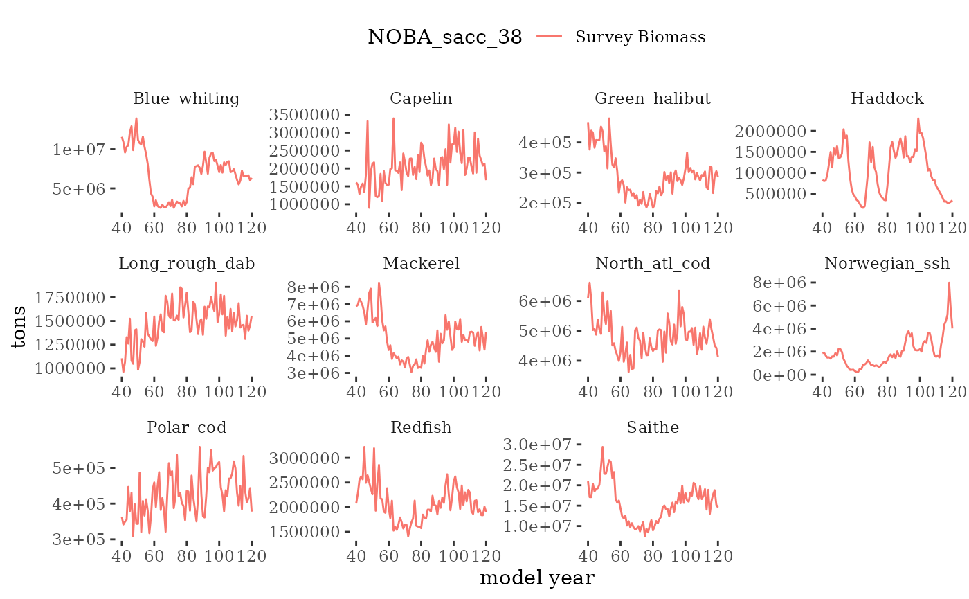
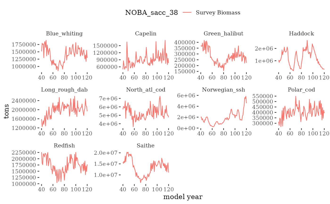
# plot biomass time series facet wrapped by species
plotB <- function(dat, truedat=NULL){
  
    svbio <- dat %>% filter(variable=="biomass")
    svcv <- dat %>% filter(variable=="cv")
  
    ggplot() +
    geom_line(data=svbio, aes(x=year,y=value, color="Survey Biomass"), 
              alpha = 10/10) +
    {if(!is.null(truedat)) geom_line(data=truedat, aes(x=time/365,y=atoutput, color="True B"), alpha = 3/10)} + 
    theme_tufte() +
    theme(legend.position = "top") +
    xlab("model year") +
    ylab("tons") +
    labs(colour=dat$ModSim) +
    facet_wrap(~Name, scales="free") 
  
}

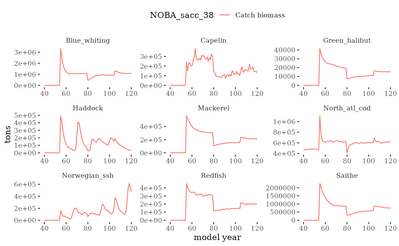
# make a catch series function that can be split by fleet? this doesnt
# also note different time (days) from model timestep in all other output
plotC <- function(dat, truedat=NULL){
  
    ctbio <- dat %>% filter(variable=="catch")
    ctcv <- dat %>% filter(variable=="cv")
  
    ggplot() +
    geom_line(data=ctbio, aes(x=year,y=value, color="Catch biomass"), 
              alpha = 10/10) +
    {if(!is.null(truedat)) geom_line(data=truedat, aes(x=time/365,y=atoutput, color="True Catch"), alpha = 3/10)} + 
    theme_tufte() +
    theme(legend.position = "top") +
    xlab("model year") +
    ylab("tons") +
    labs(colour=dat$ModSim) +
    facet_wrap(~Name, scales="free") 
  
}

# note on ggplot default colors, can get the first and second using this
# library(scales)
# show_col(hue_pal()(2))

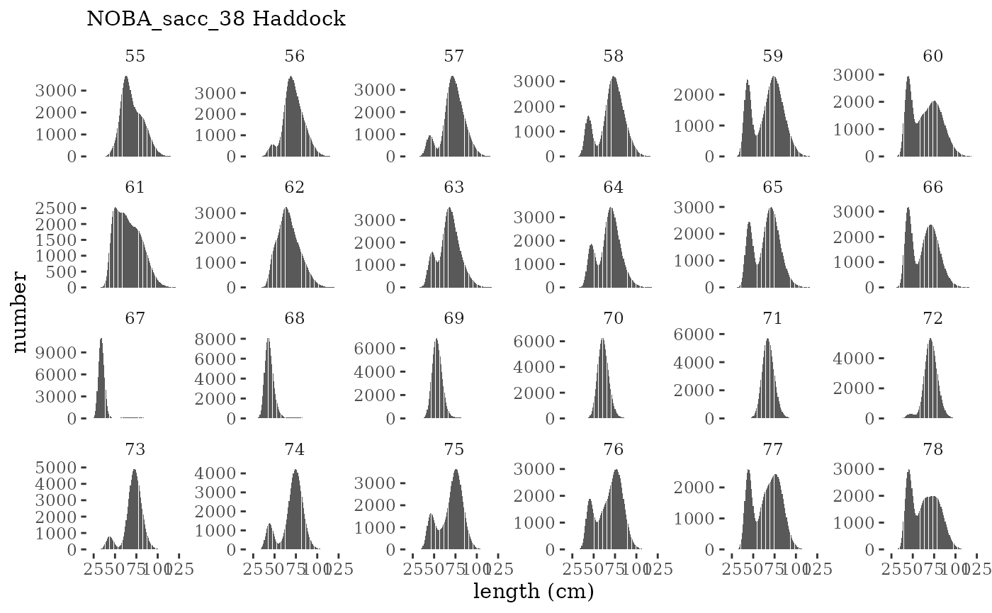
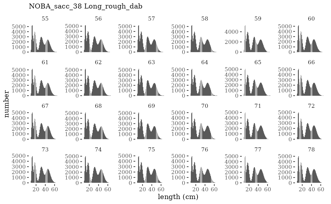
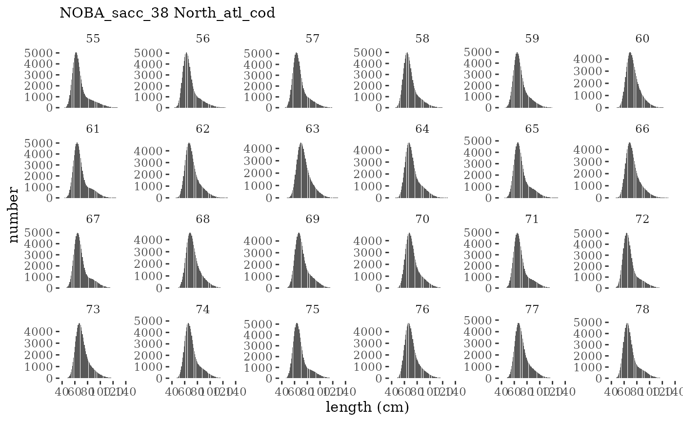
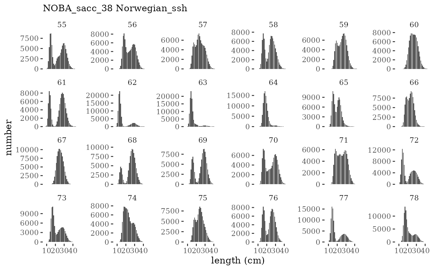
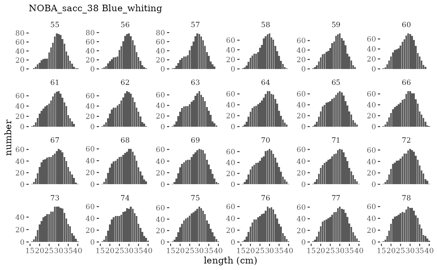
# plot length frequencies by timestep (one species)
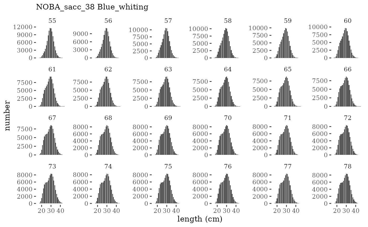
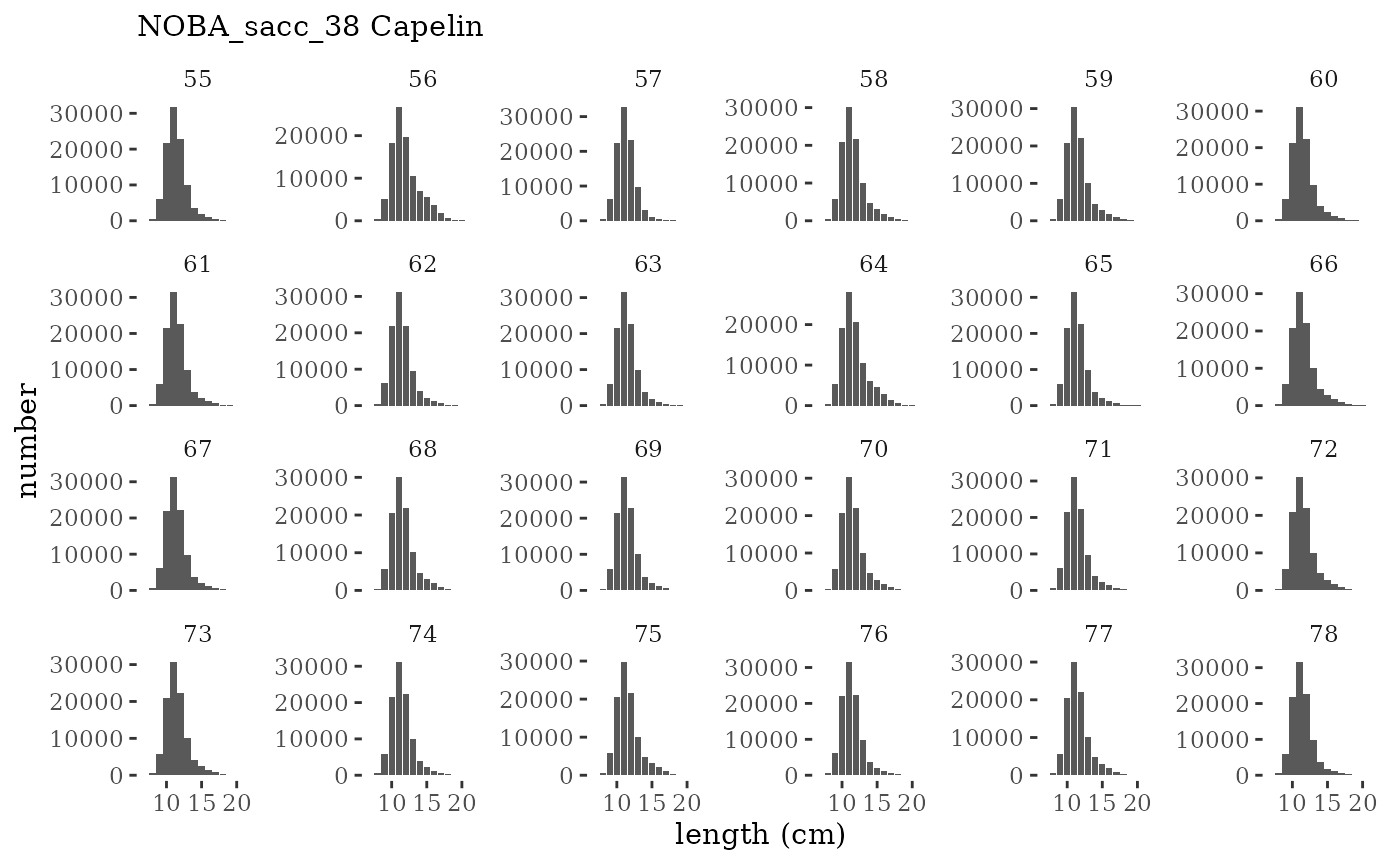
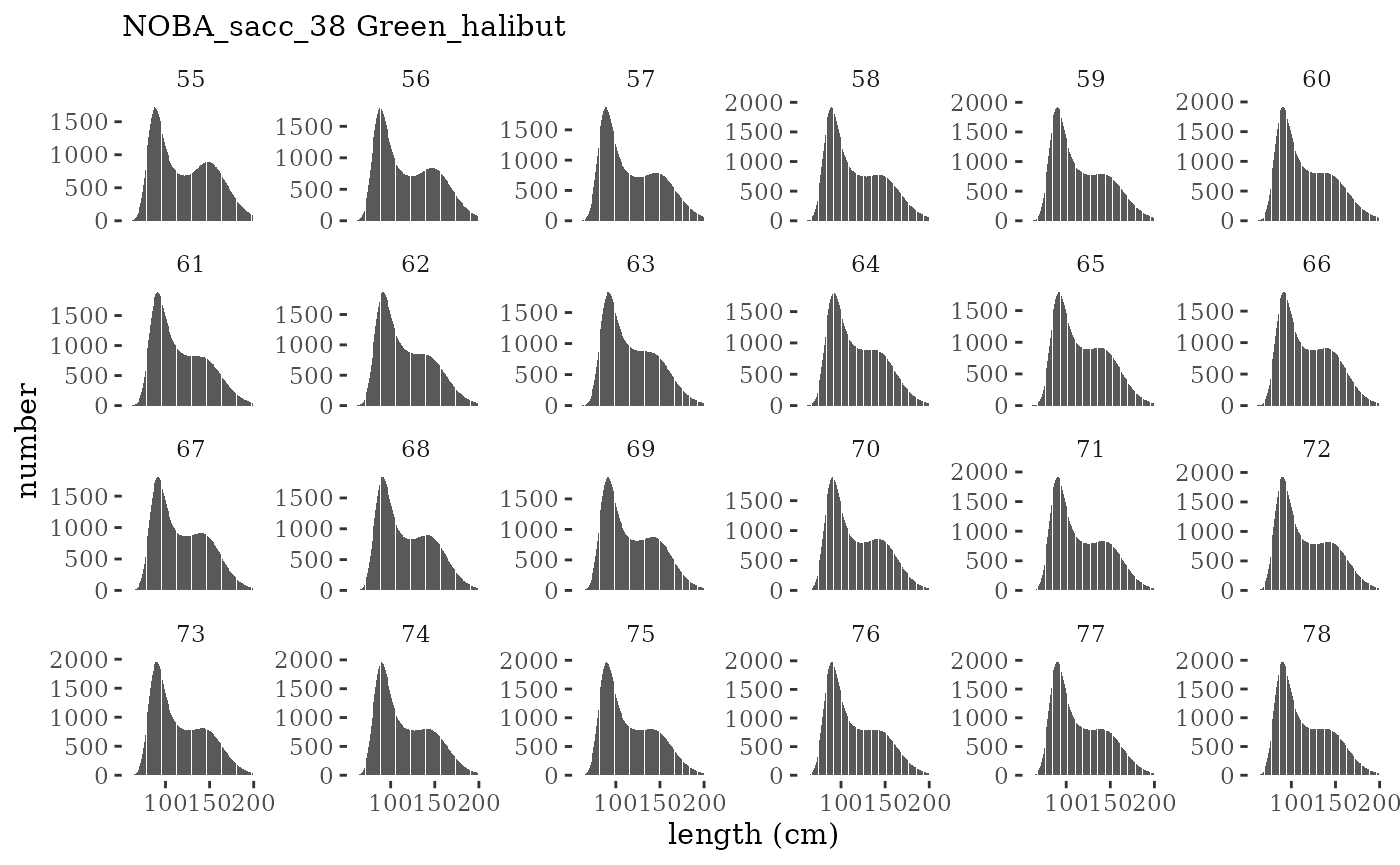
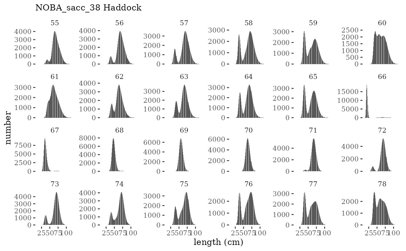
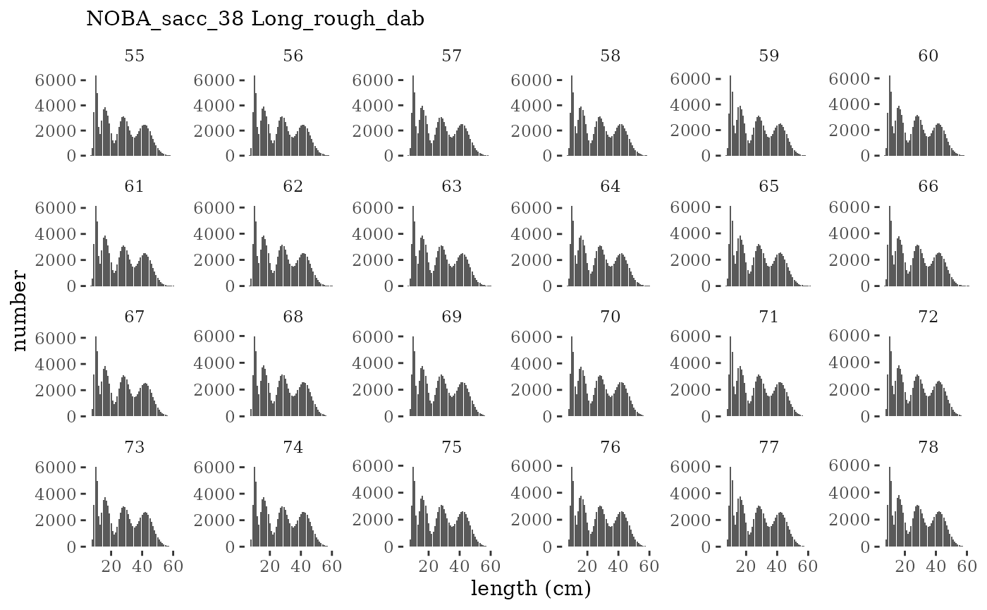
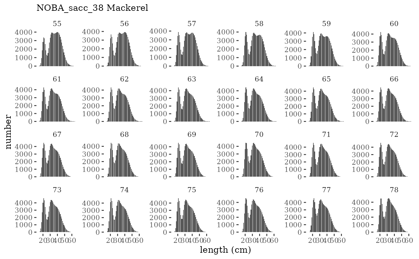
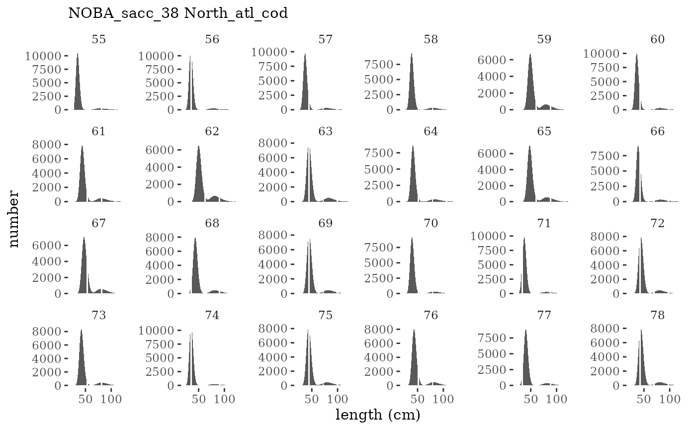
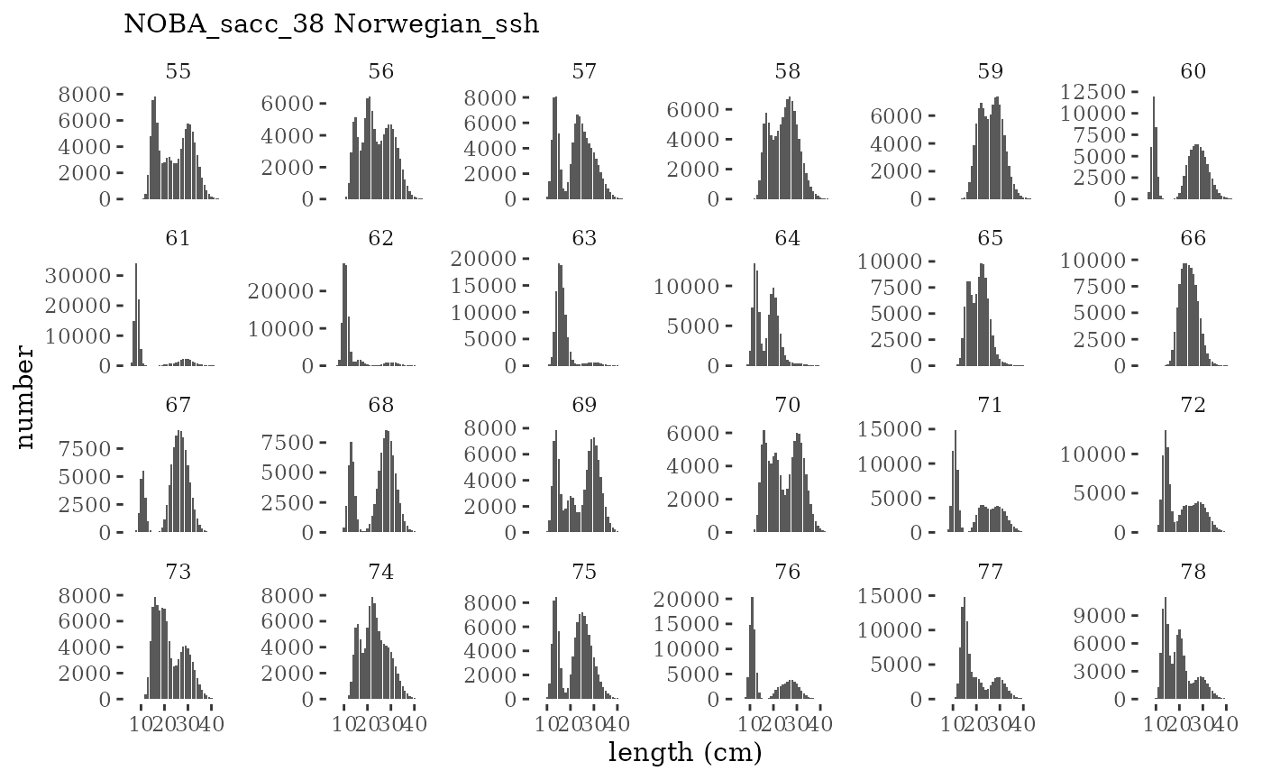
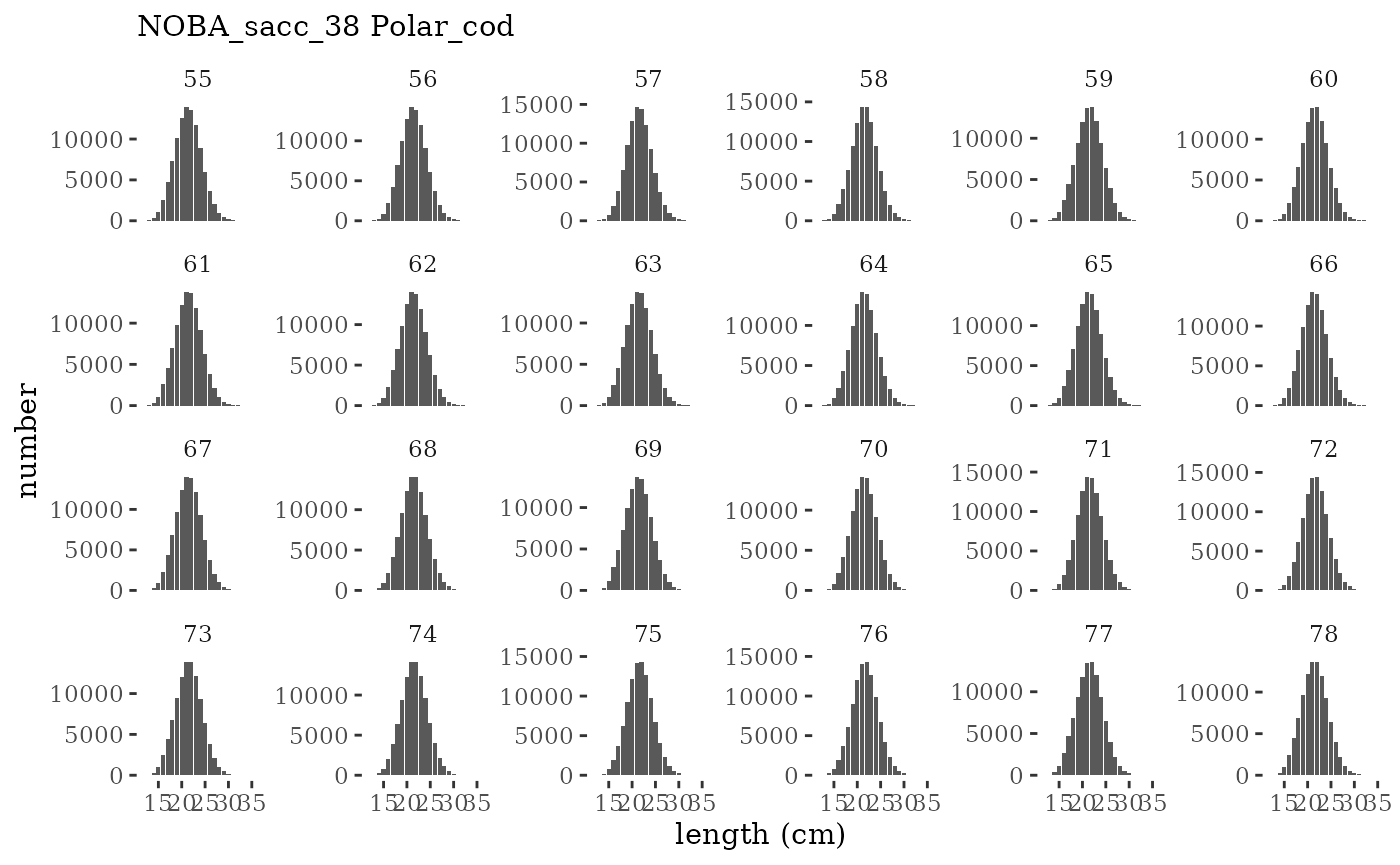
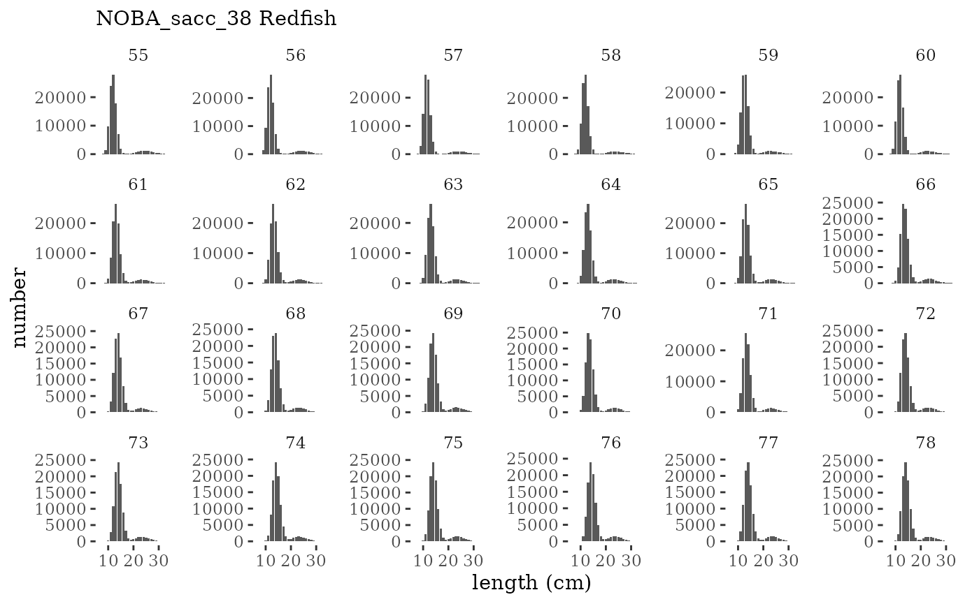
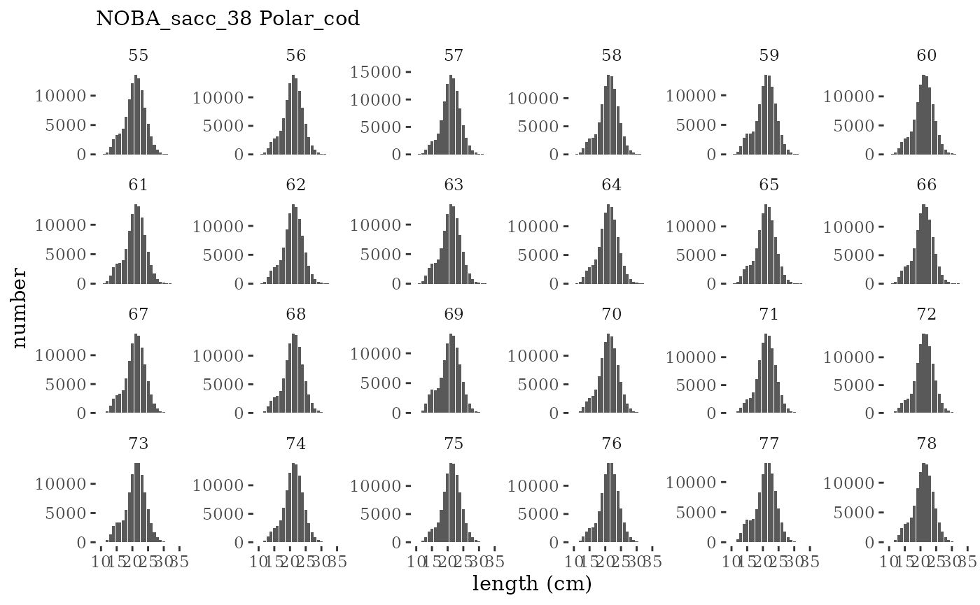
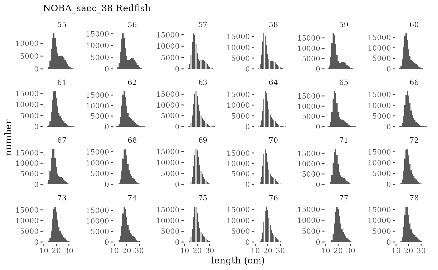
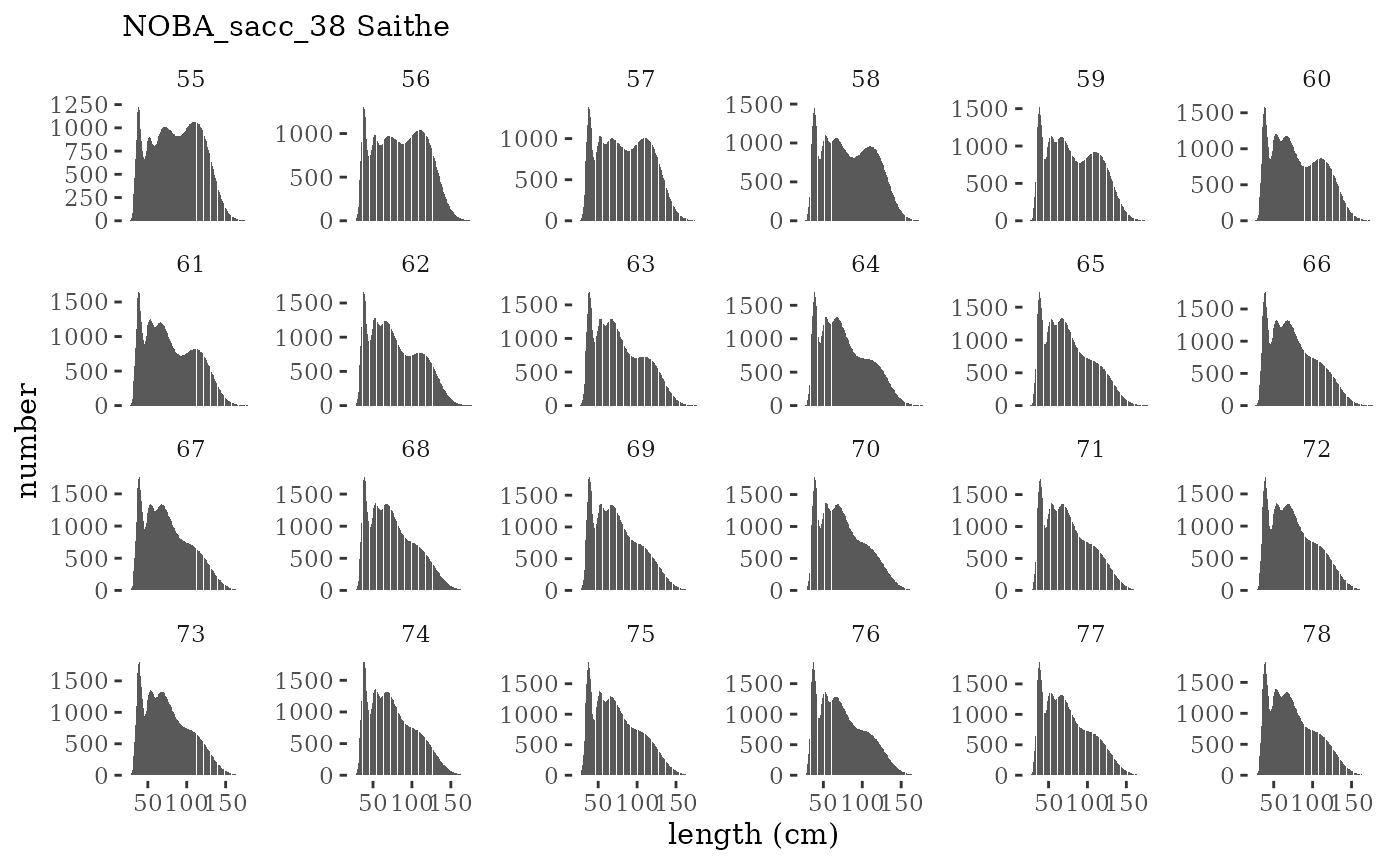
plotlen <- function(dat, effN=1, truedat=NULL){
  
  cols <- c("Census Lcomp"="#00BFC4","Sample Lcomp"="#F8766D")  
  ggplot(mapping=aes(x=lenbin)) +
    {if(is.null(truedat)) geom_bar(data=dat, aes(weight = value/effN))} +
    {if(!is.null(truedat)) geom_bar(data=dat, aes(weight = censuslen/totlen, fill="Census Lcomp"), alpha = 5/10)} +
    {if(!is.null(truedat)) geom_bar(data=dat, aes(weight = atoutput/effN, fill="Sample Lcomp"), alpha = 5/10)} +
    theme_tufte() +
    theme(legend.position = "bottom") +
    xlab("length (cm)") +
    {if(is.null(truedat)) ylab("number")} +
    {if(!is.null(truedat)) ylab("proportion")} +
    scale_colour_manual(name="", values=cols) +
    labs(subtitle = paste(dat$ModSim,
                          dat$Name)) +
    facet_wrap(~year, ncol=6, scales="free_y")

}

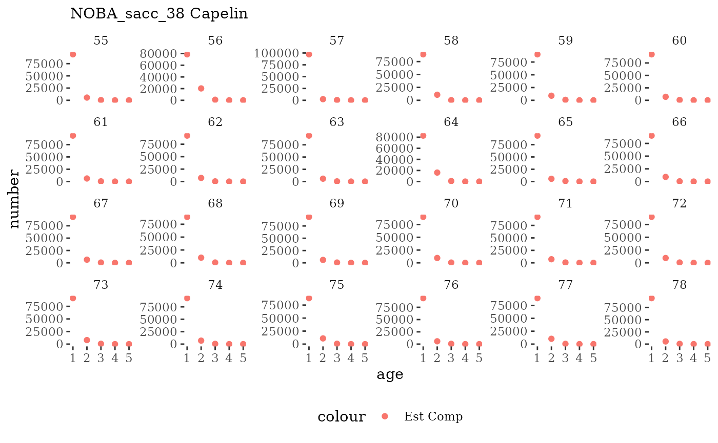
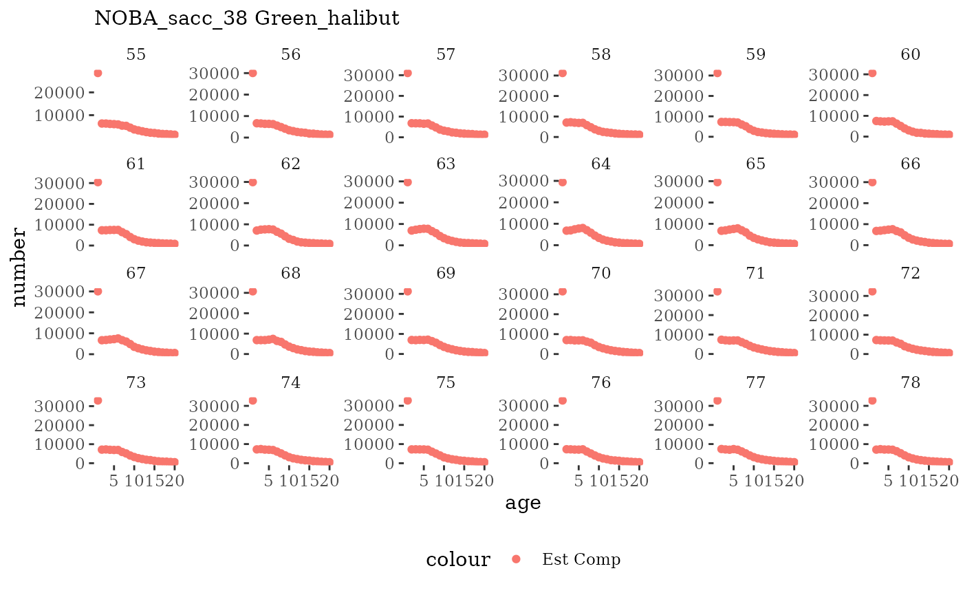
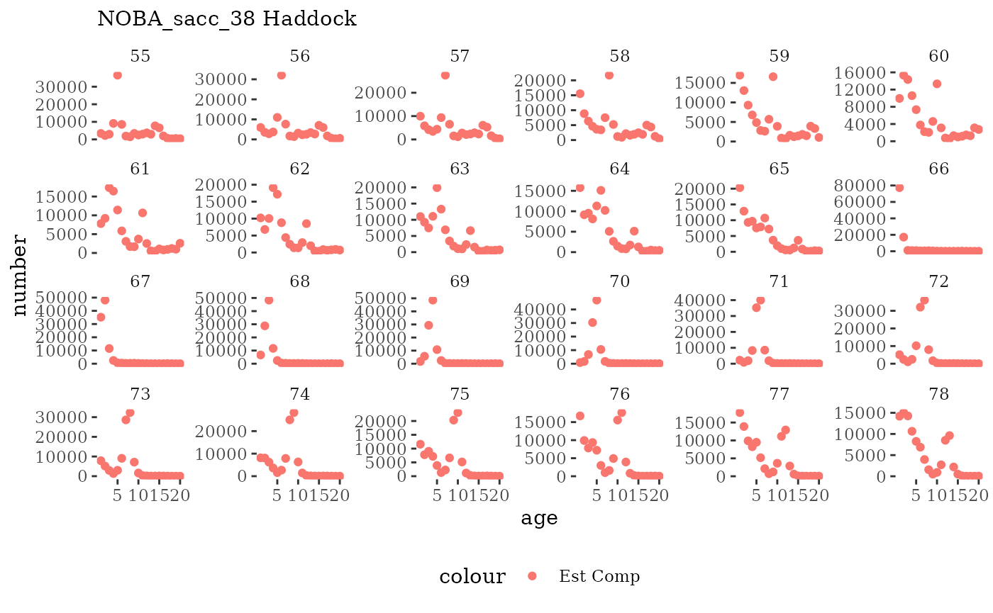
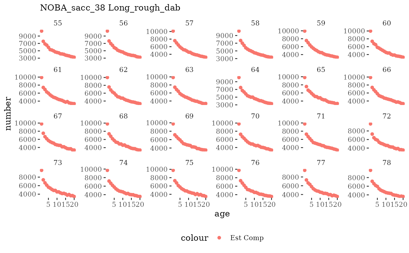
# plot numbers at age by timestep (one species)
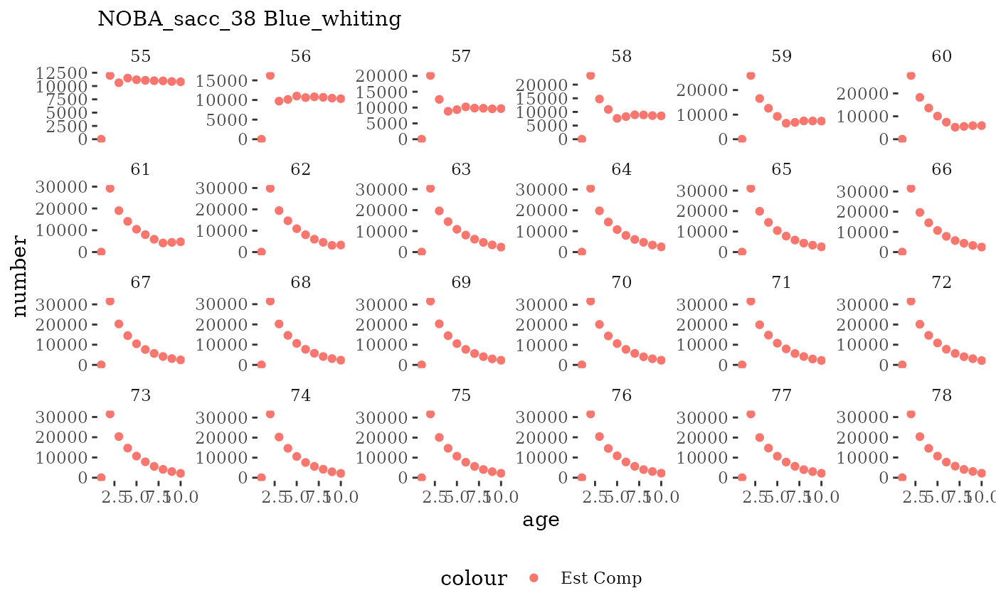
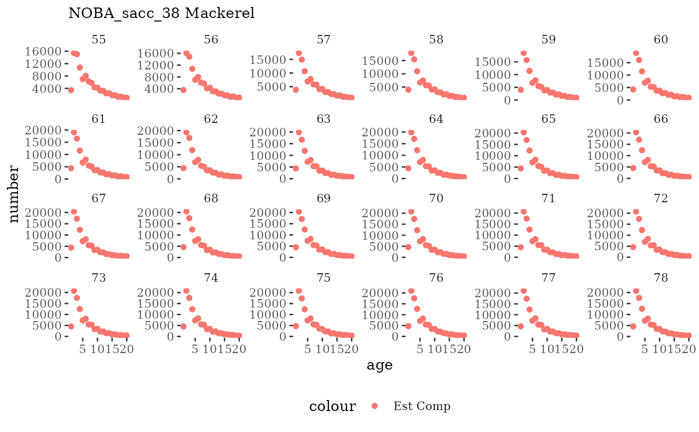
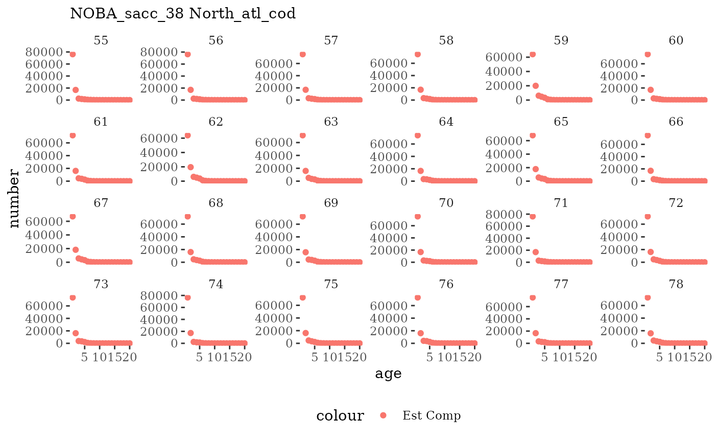
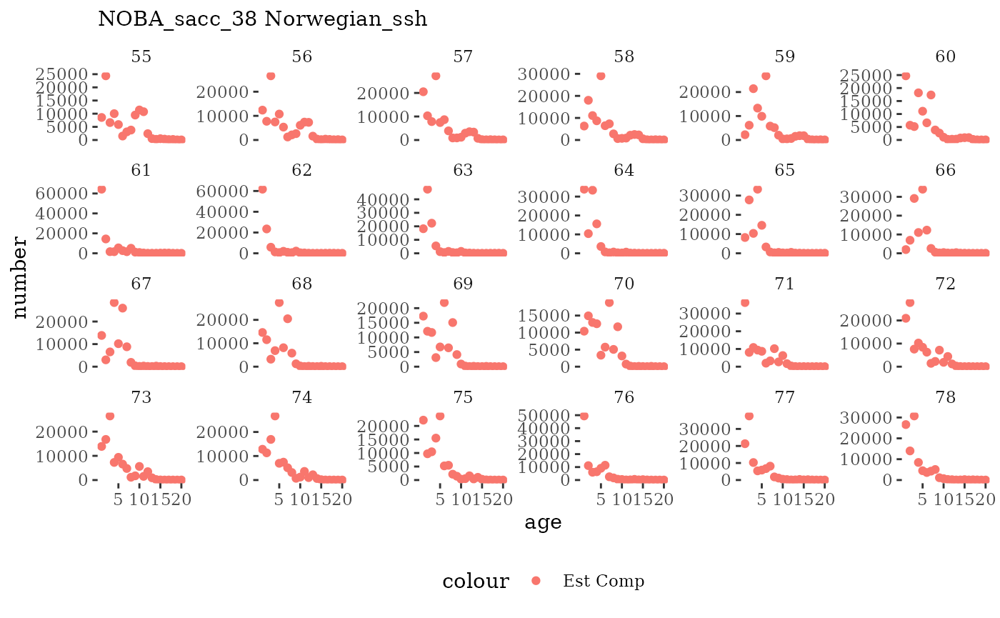
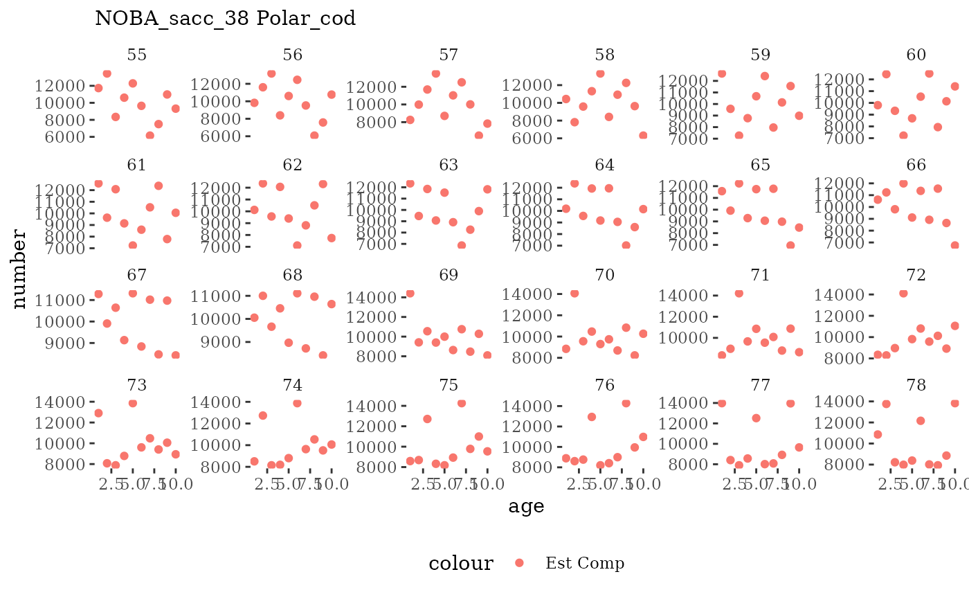
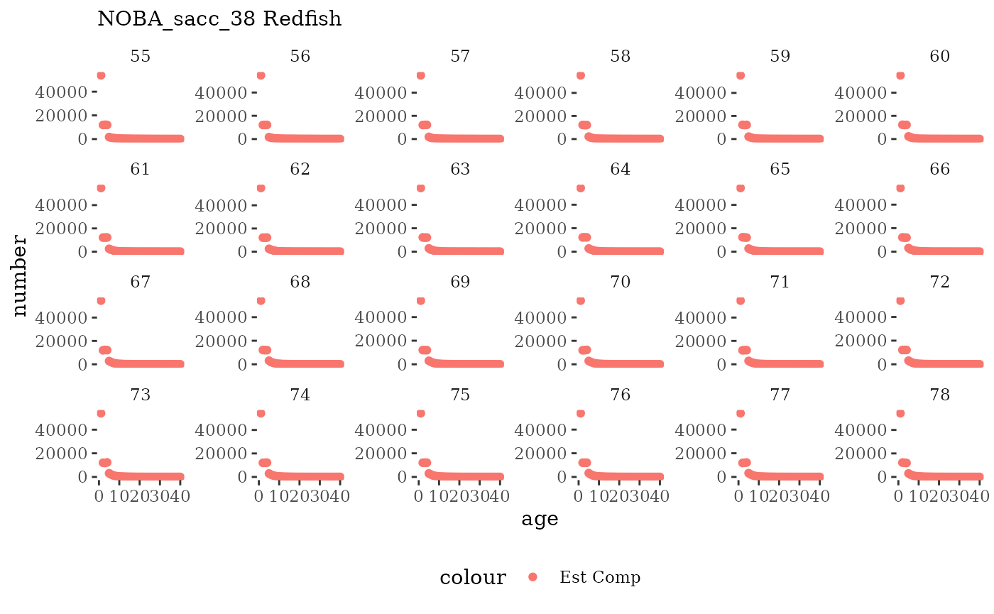
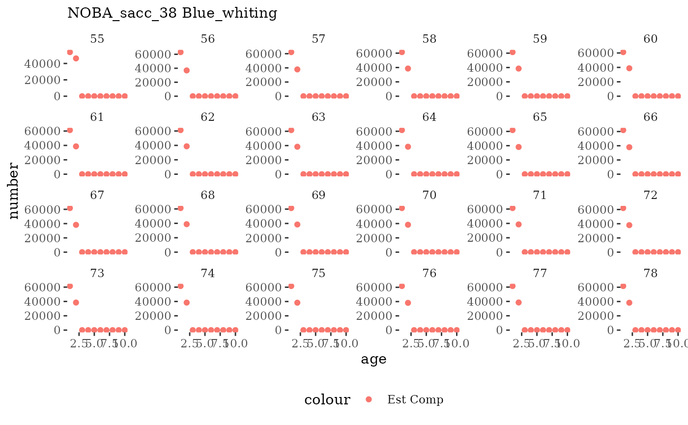
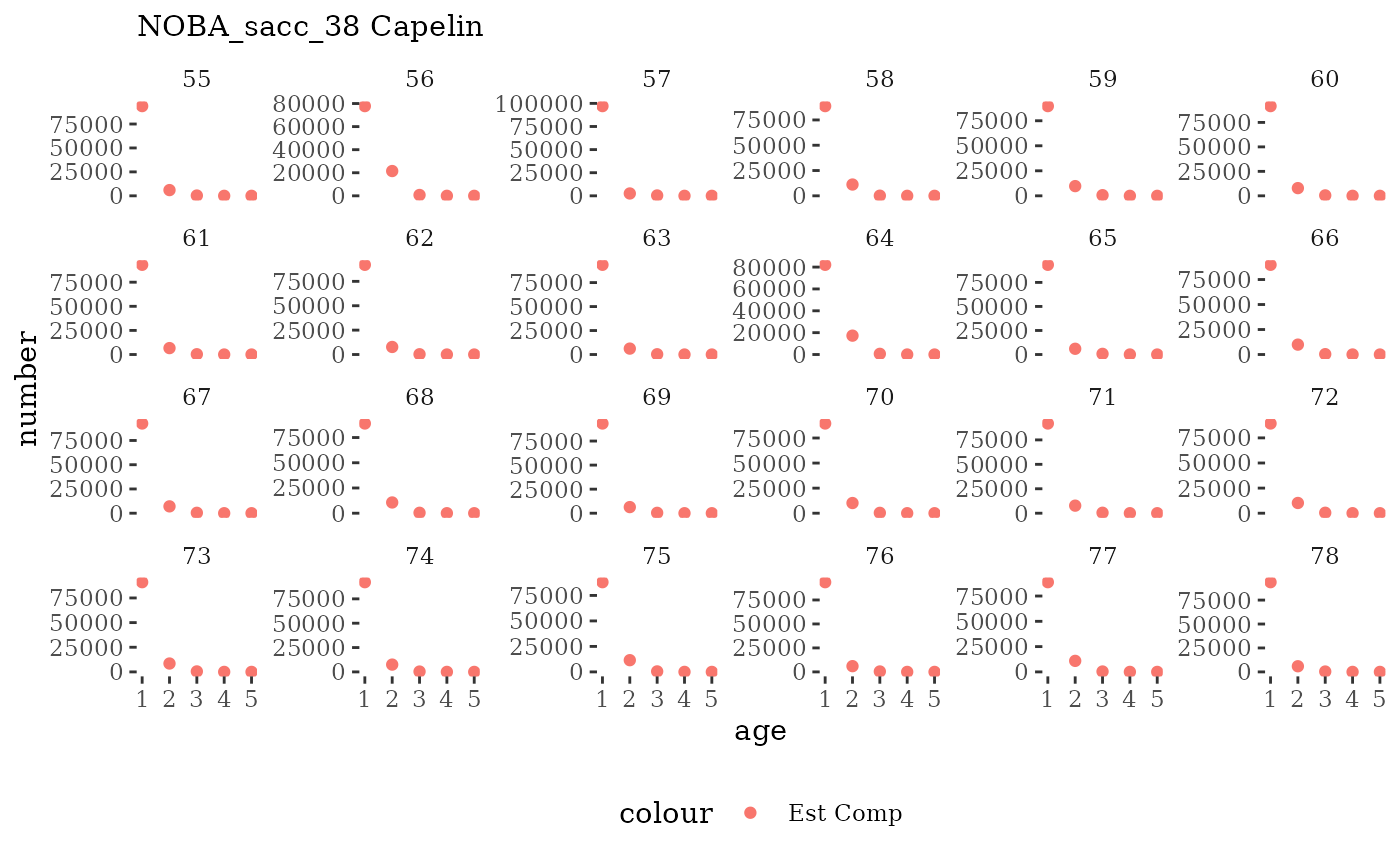
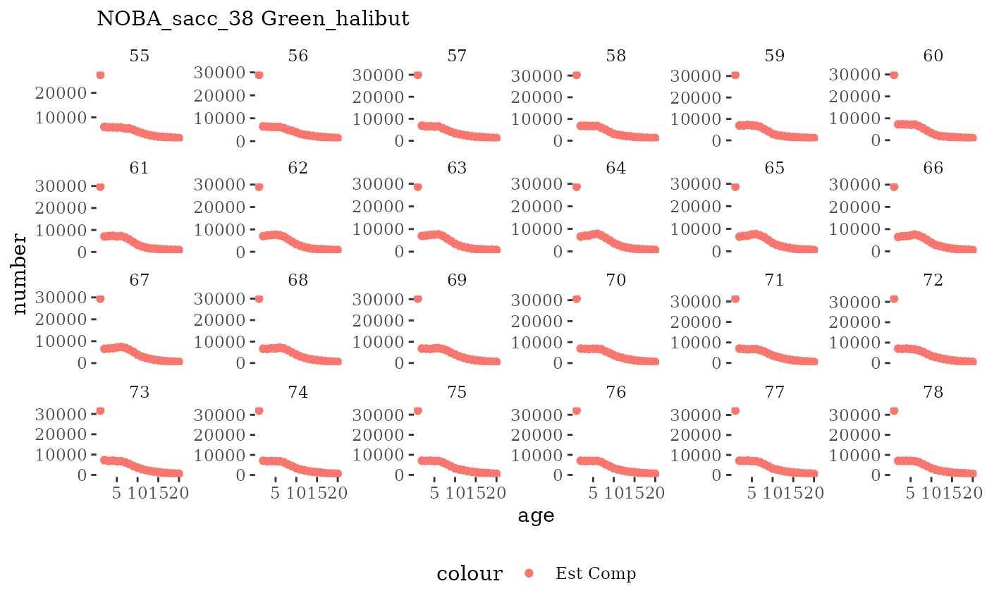
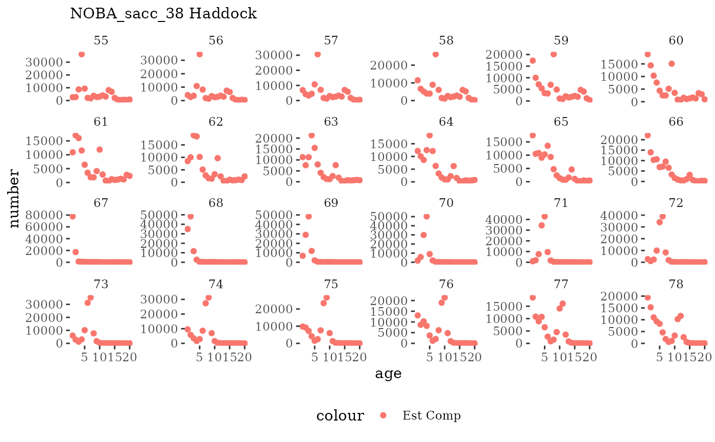
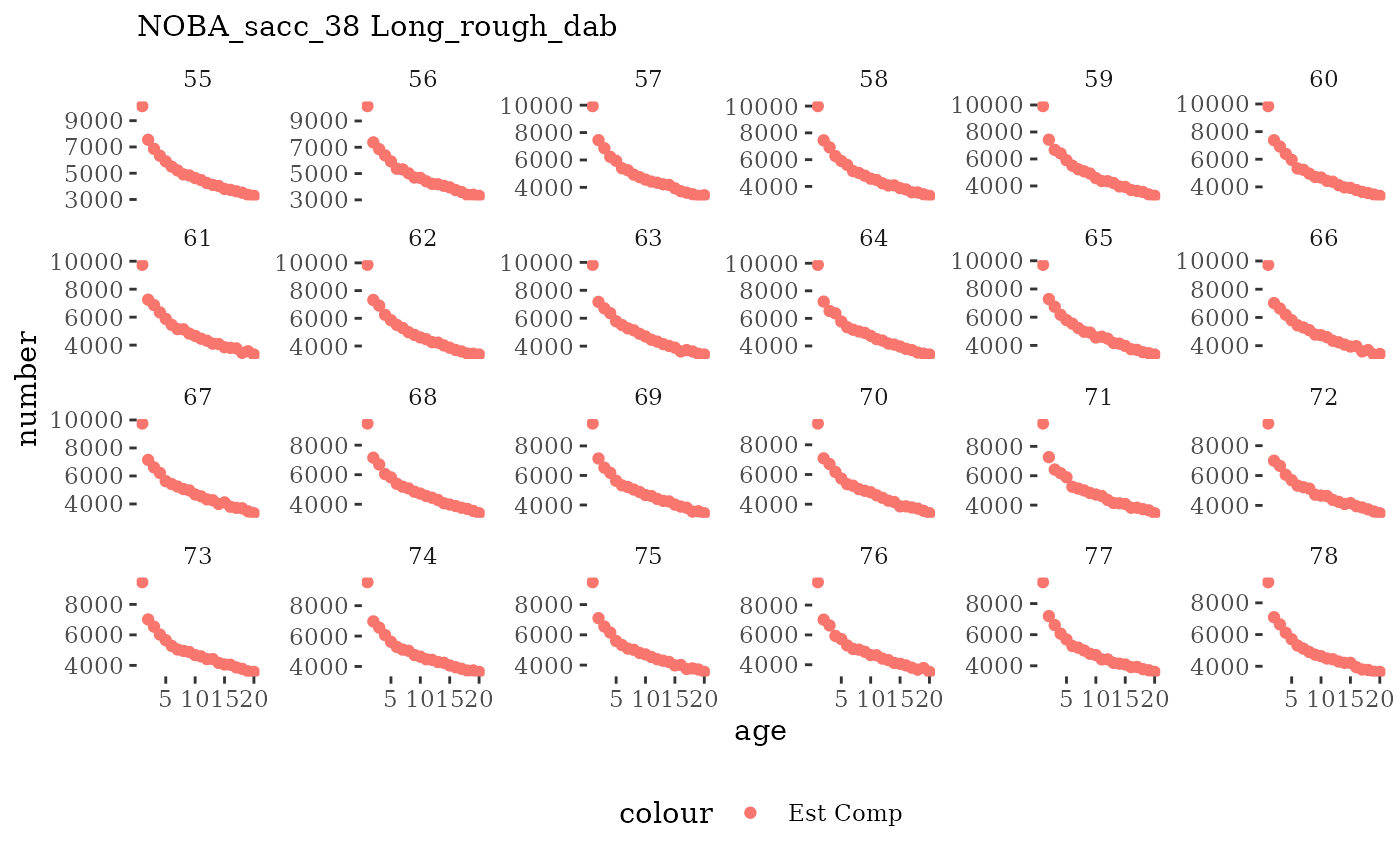
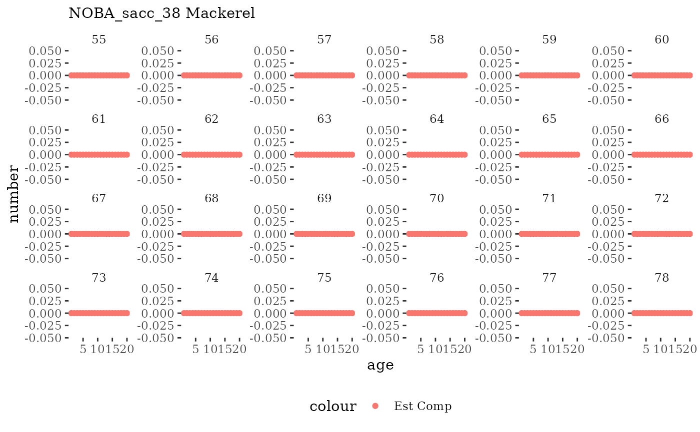
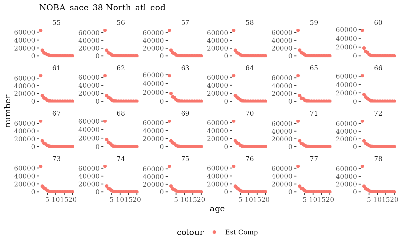
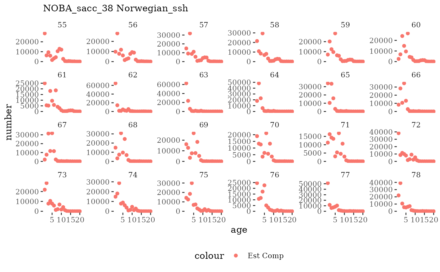
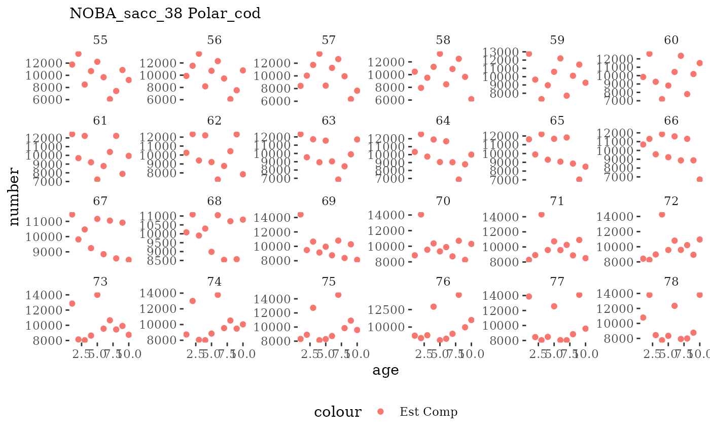
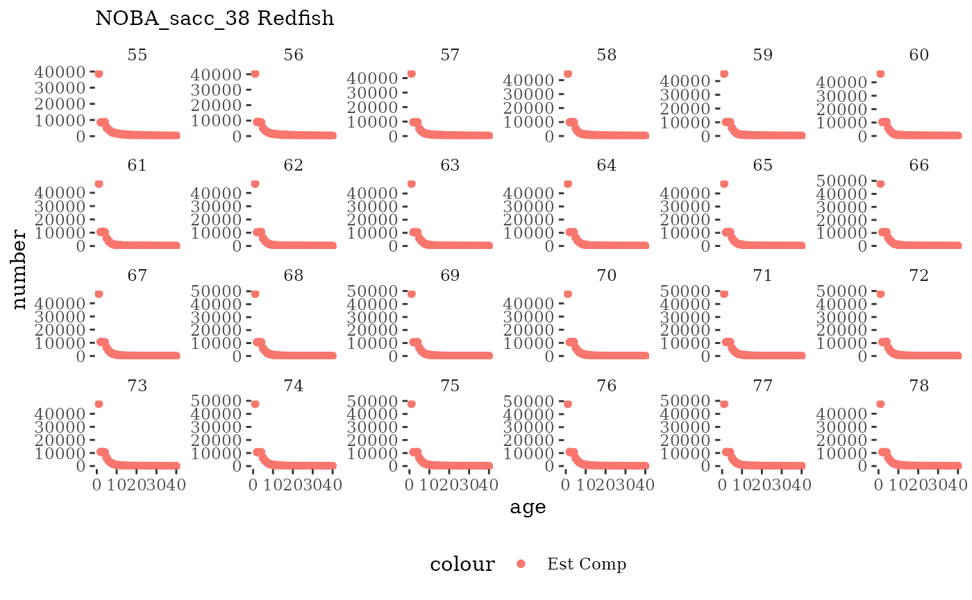
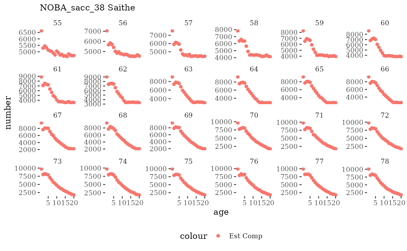
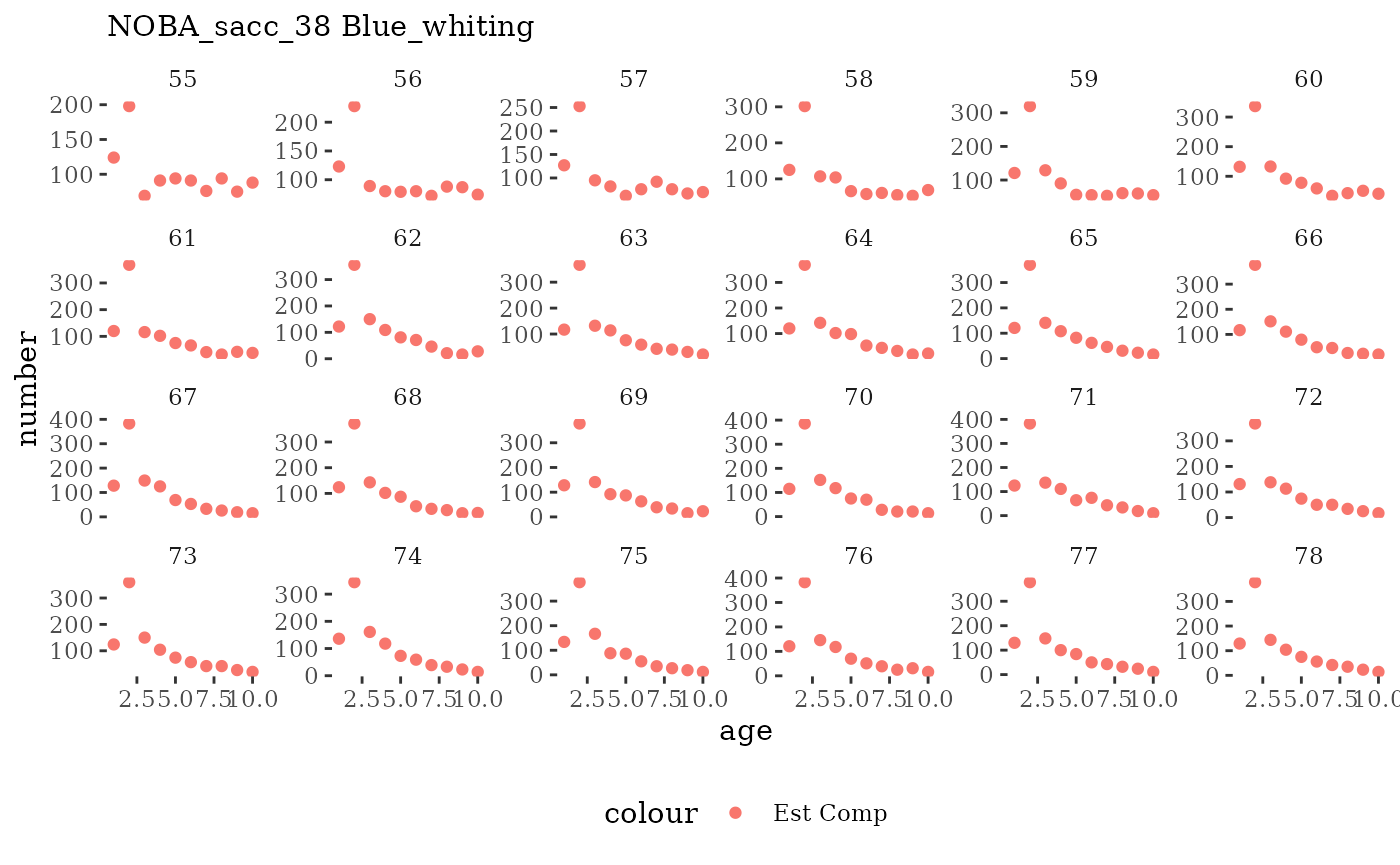
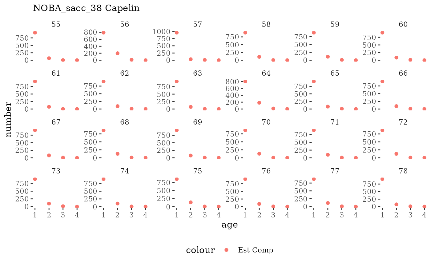
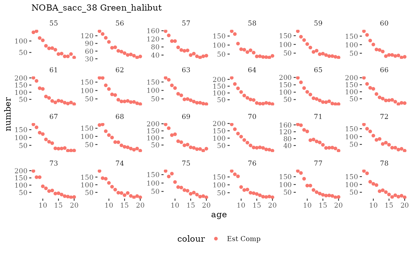
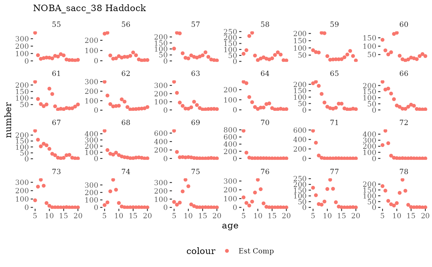
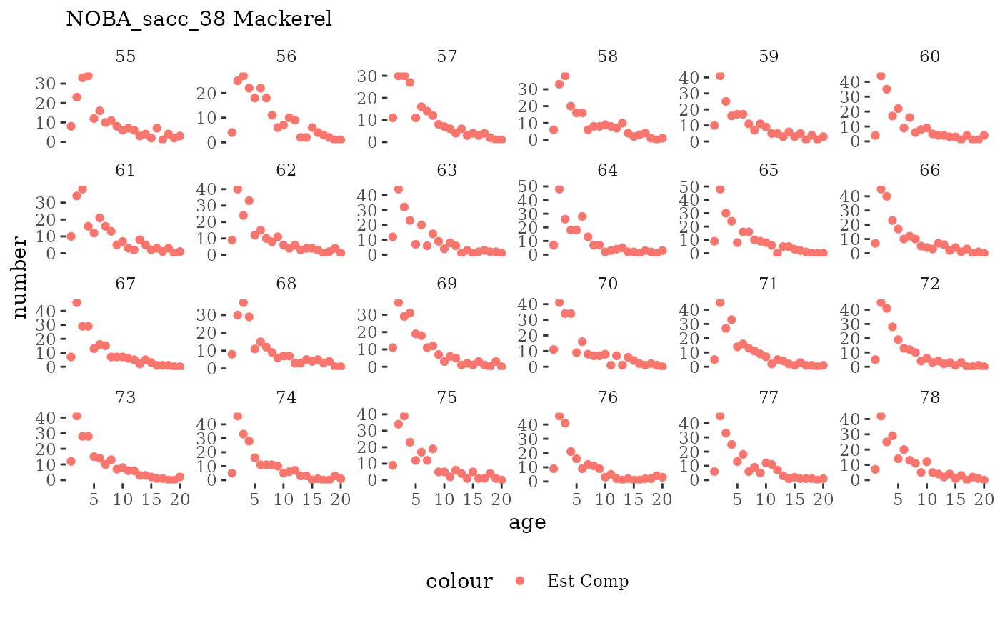
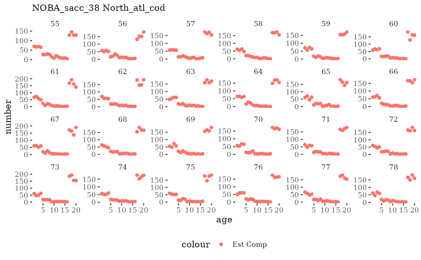
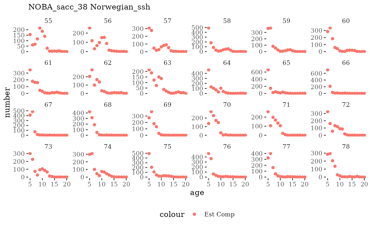
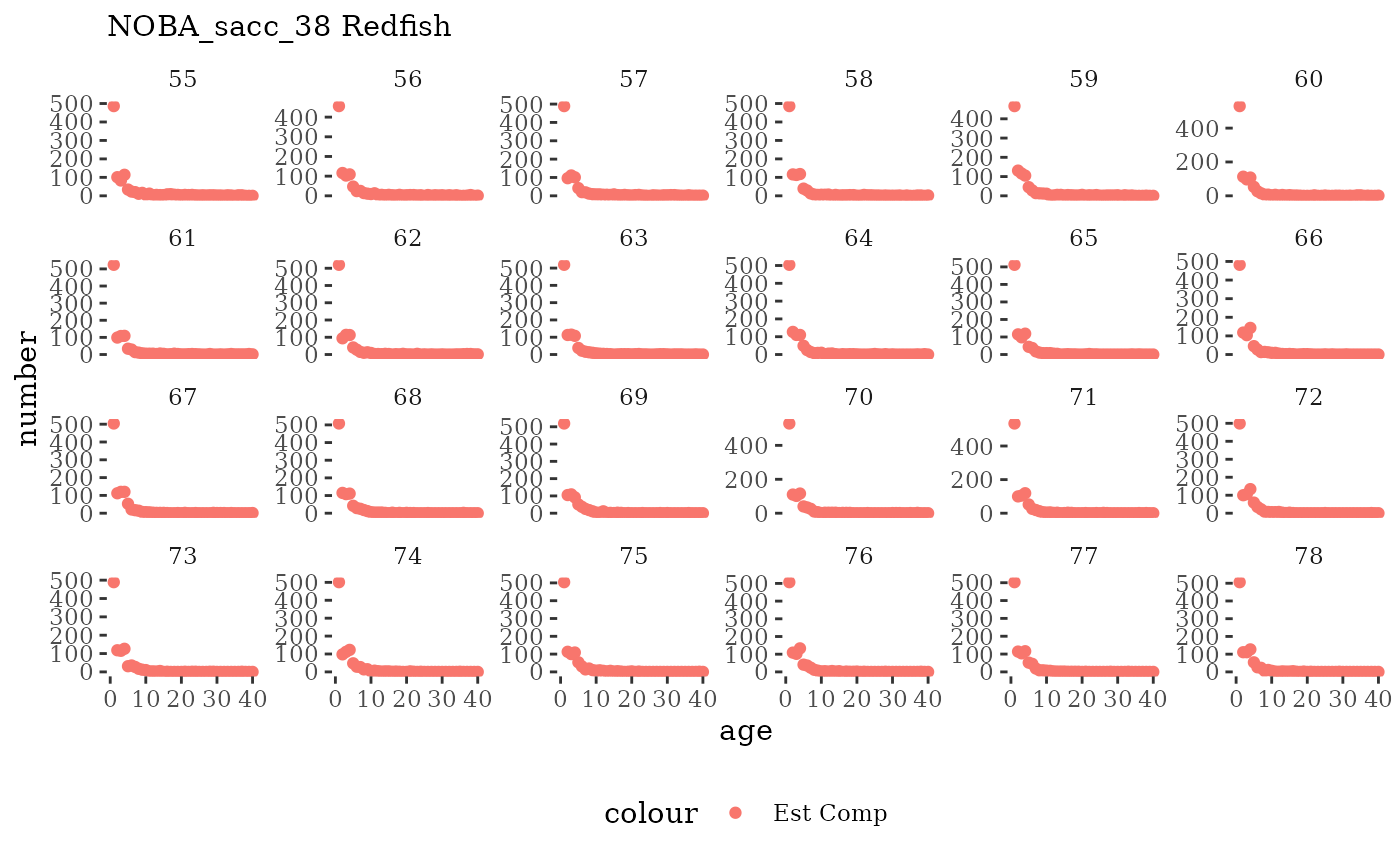
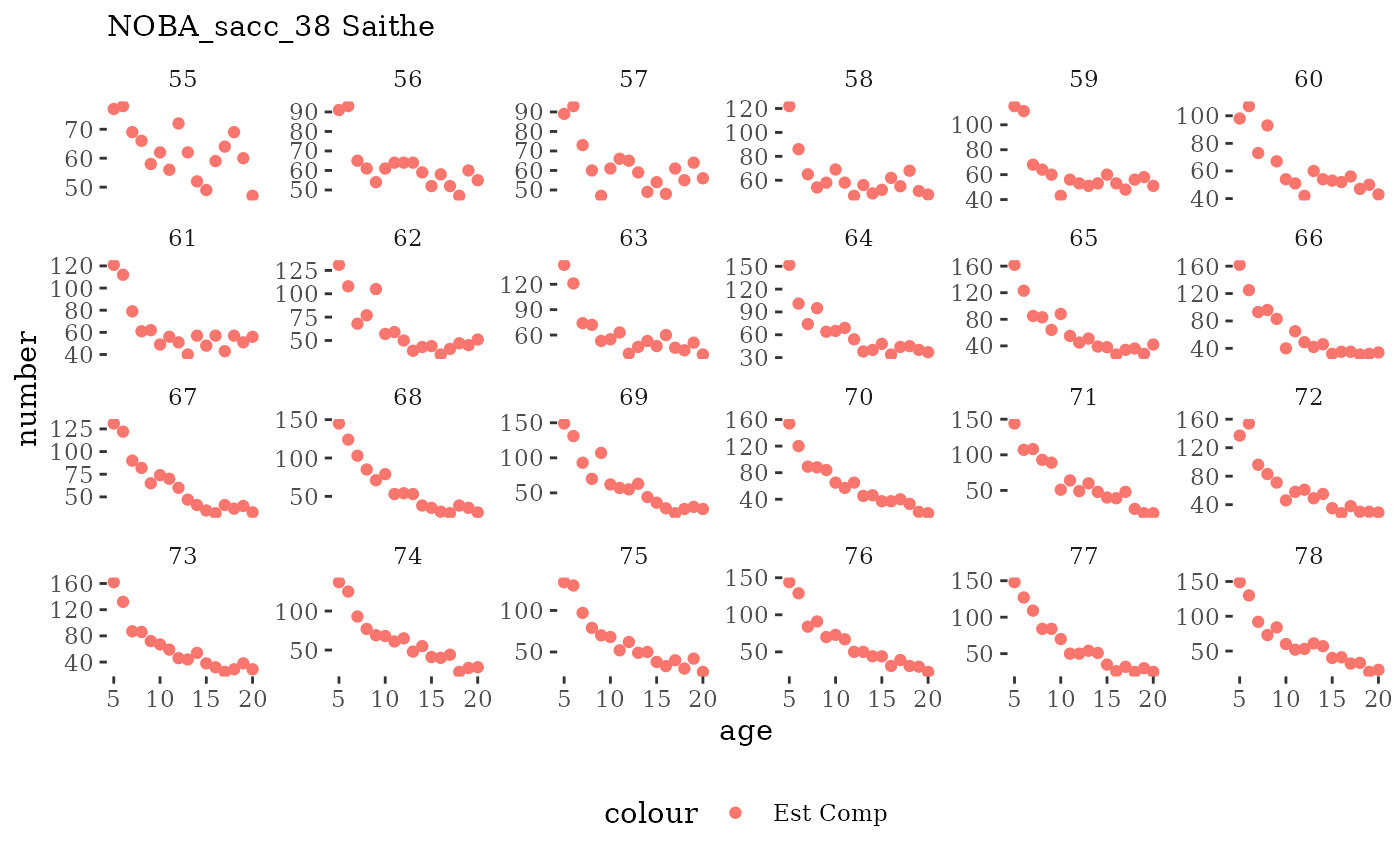
Natageplot <- function(dat, effN=1, truedat=NULL){
  ggplot() +
    geom_point(data=dat, aes(x=age, y=value/effN, color="Est Comp")) +
    {if(!is.null(truedat)) geom_line(data=dat, aes(x=agecl, y=numAtAge/totN, color="True Comp"))} + 
    theme_tufte() +
    theme(legend.position = "bottom") +    
    xlab("age") +
    {if(is.null(truedat)) ylab("number")} +
    {if(!is.null(truedat)) ylab("proportion")} +
    labs(subtitle = paste(dat$ModSim,
                          dat$Name)) + 
    facet_wrap(~year, ncol=6, scales="free_y")
}

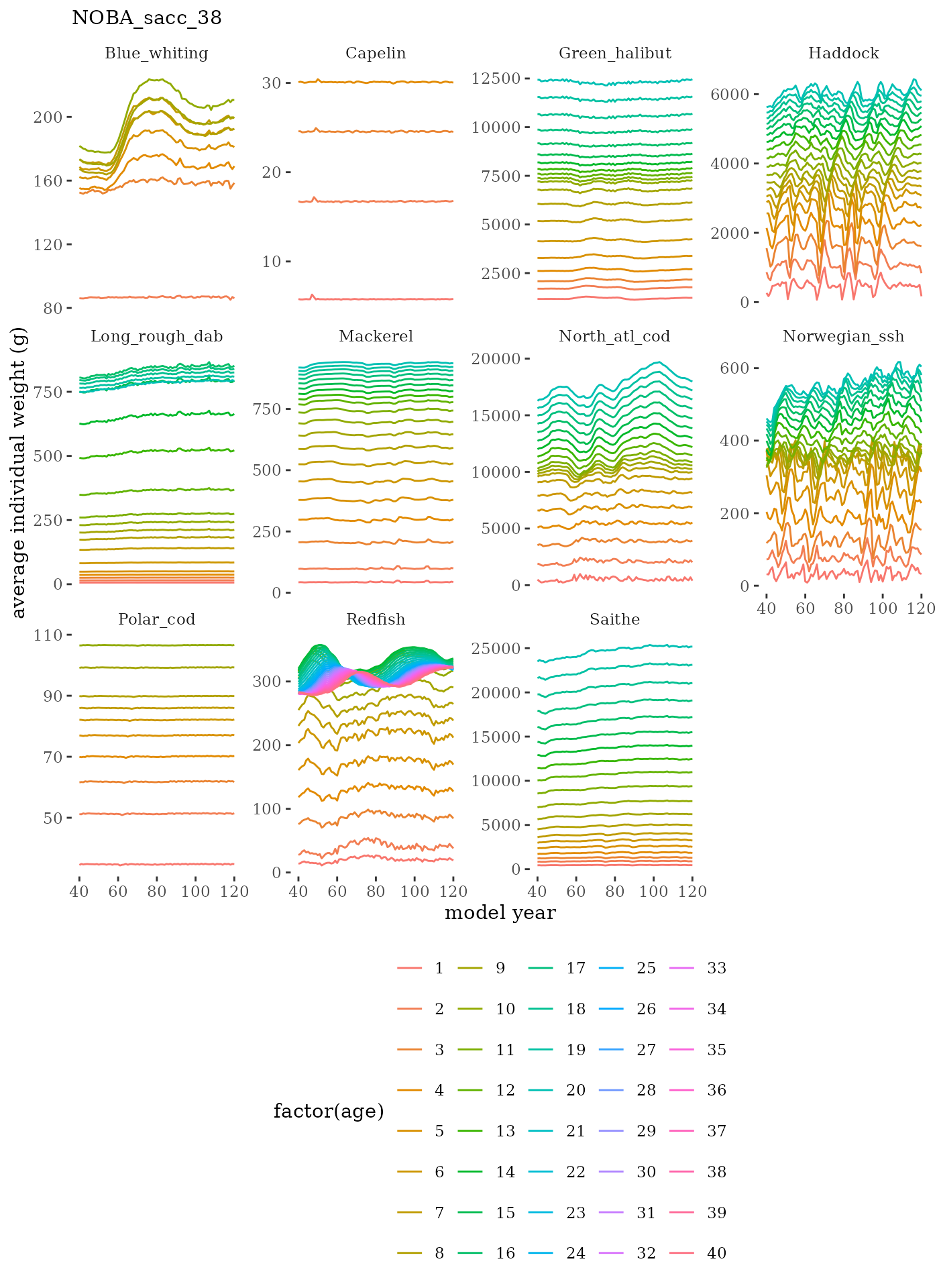
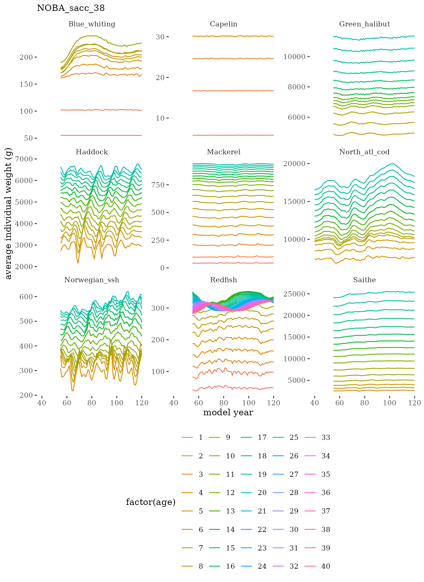
# plot weight at age time series facet wrapped by species
wageplot <- function(dat, truedat=NULL){
  ggplot(dat, aes(year, value)) +
    geom_line(aes(colour = factor(age))) +
    theme_tufte() +
    theme(legend.position = "bottom") +
    xlab("model year") +
    ylab("average individual weight (g)") +
    labs(subtitle = paste0(dat$ModSim)) +
    facet_wrap(c("Name"), scales="free_y")
}

Read in the “data” to check with plots

The mskeyrun simulated data objects are all dataframes.

survObsBiom <- mskeyrun::simSurveyIndex #atlantisom::read_savedsurvs(d.name, 'survB')
#age_comp_data <- mskeyrun::simSurveyAgeLencomp #atlantisom::read_savedsurvs(d.name, 'survAge') #not using in assessment
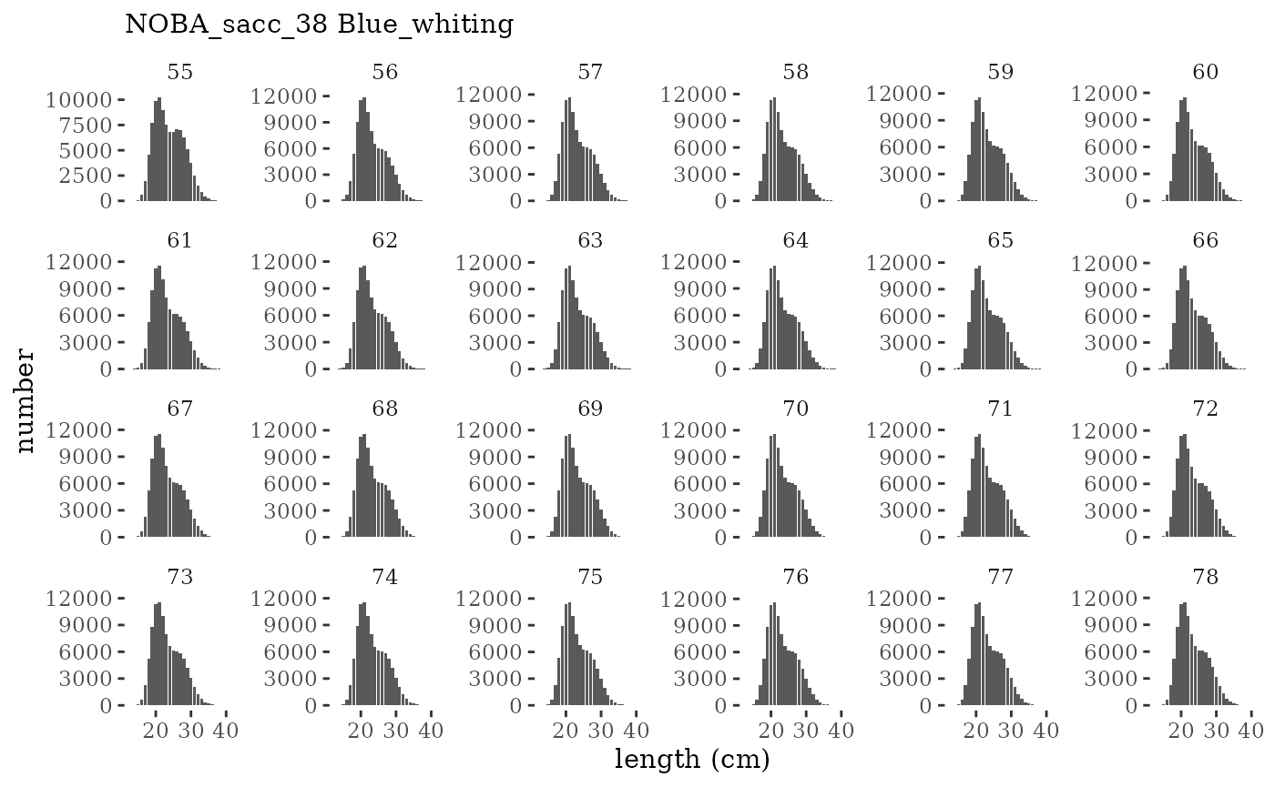
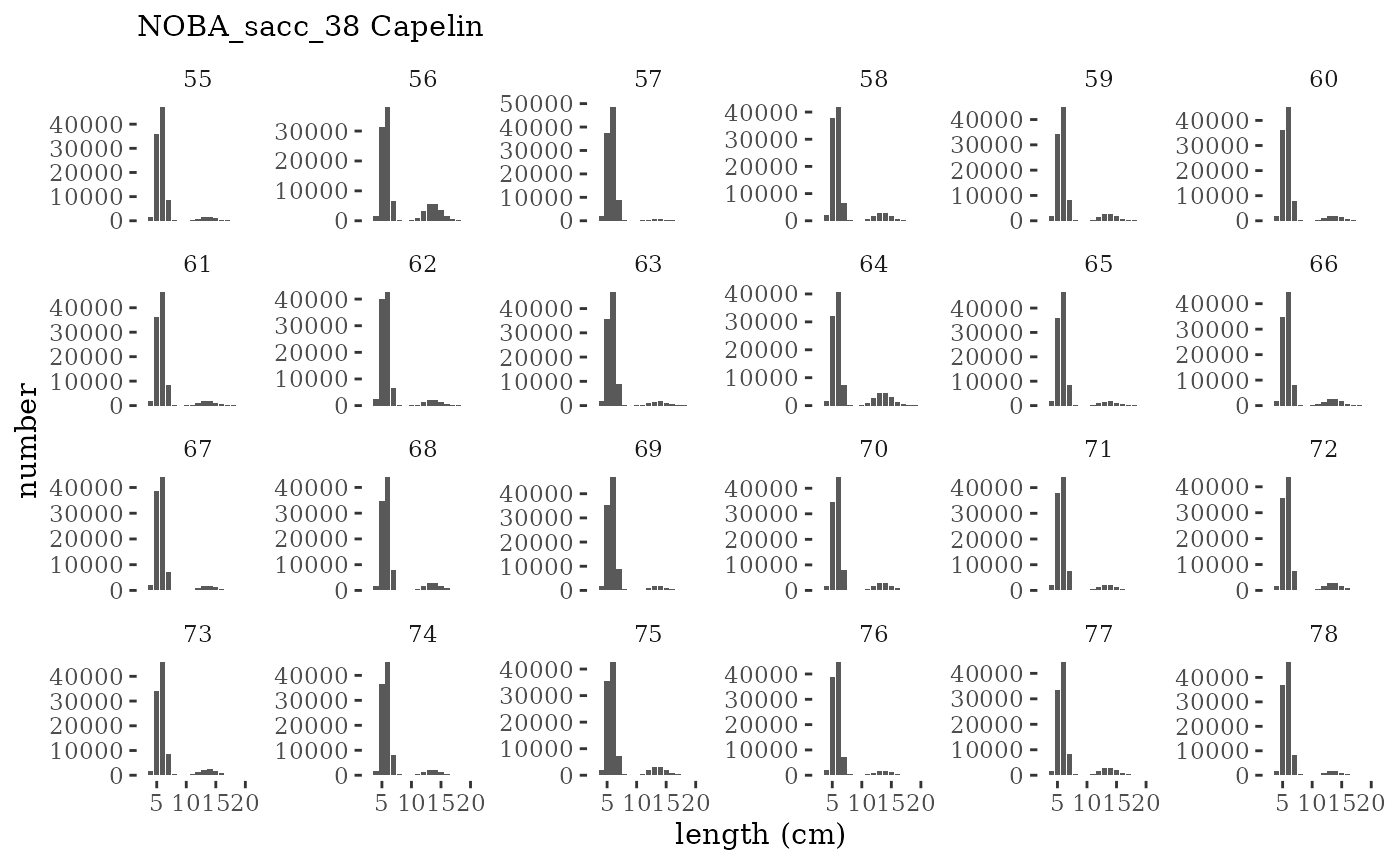
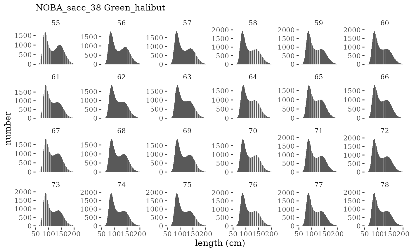
len_comp_data <- mskeyrun::simSurveyLencomp #atlantisom::read_savedsurvs(d.name, 'survLen')
#wtage <- atlantisom::read_savedsurvs(d.name, 'survWtage')  #not using in assessment
annage_comp_data <- mskeyrun::simSurveyAgecomp #atlantisom::read_savedsurvs(d.name, 'survAnnAge')
annage_wtage <- mskeyrun::simSurveyWtatAge #atlantisom::read_savedsurvs(d.name, 'survAnnWtage')

#all_diets <- atlantisom::read_savedsurvs(d.name, 'survDiet') #not using in assessment

catchbio_ss <- mskeyrun::simCatchIndex #atlantisom::read_savedfisheries(d.name, 'Catch')
catchlen_ss <- mskeyrun::simFisheryLencomp #atlantisom::read_savedfisheries(d.name, "catchLen")
#fish_age_comp <- #atlantisom::read_savedfisheries(d.name, "catchAge")
fish_annage_comp <- mskeyrun::simFisheryAgecomp #atlantisom::read_savedfisheries(d.name, 'catchAnnAge')
fish_annage_wtage <- mskeyrun::simFisheryWtatAge #atlantisom::read_savedfisheries(d.name, 'catchAnnWtage')

Visualize survey outputs

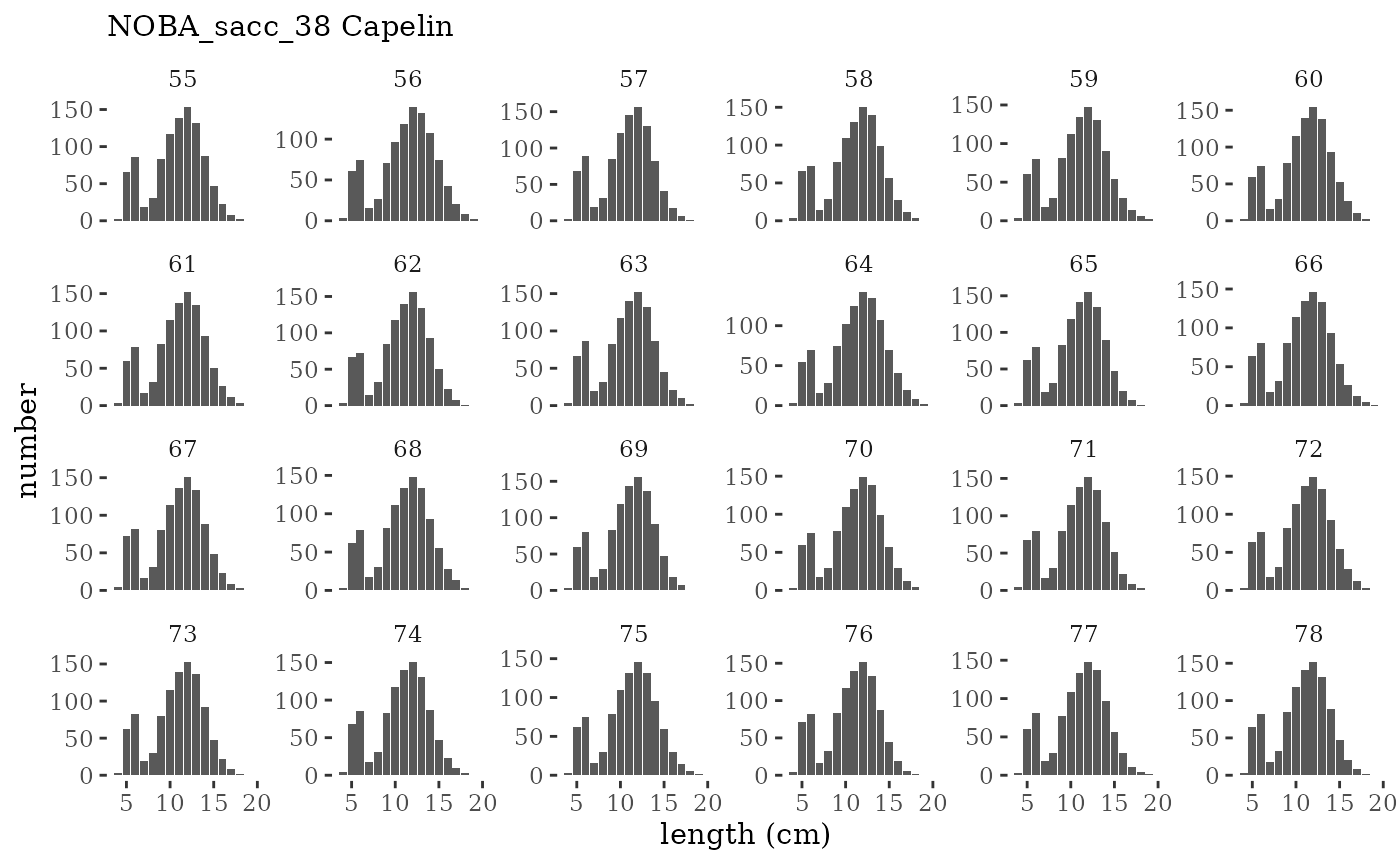
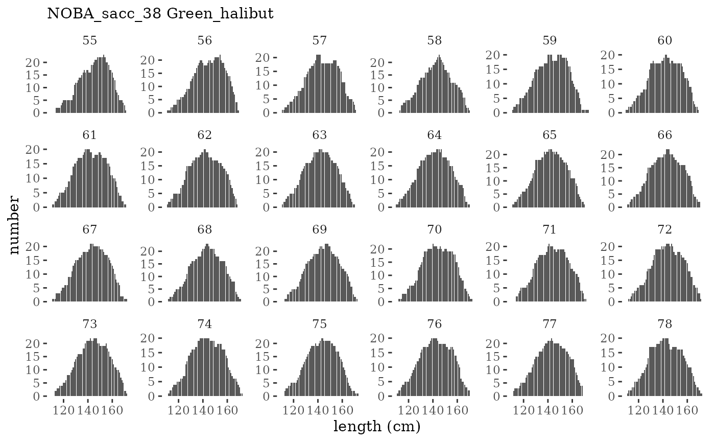
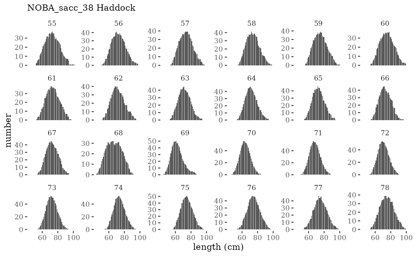
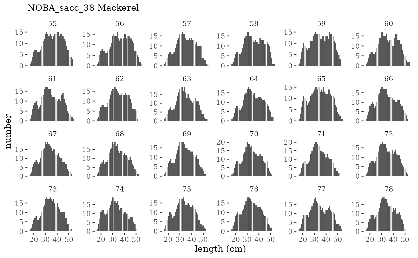
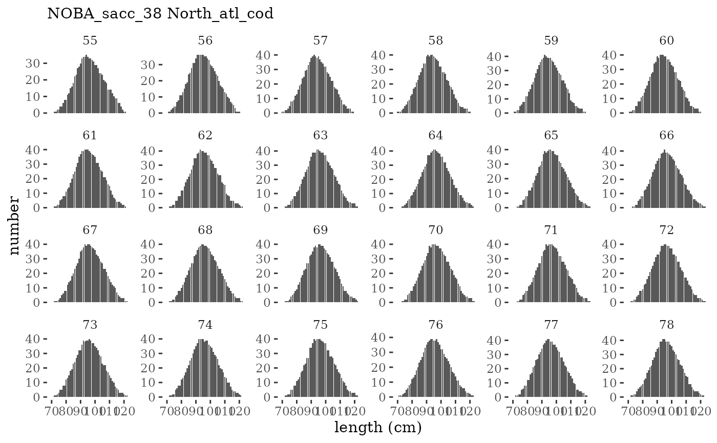
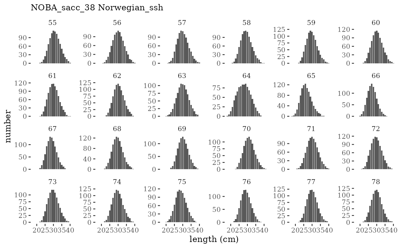
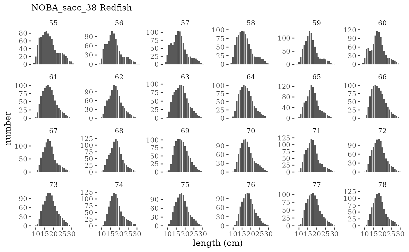
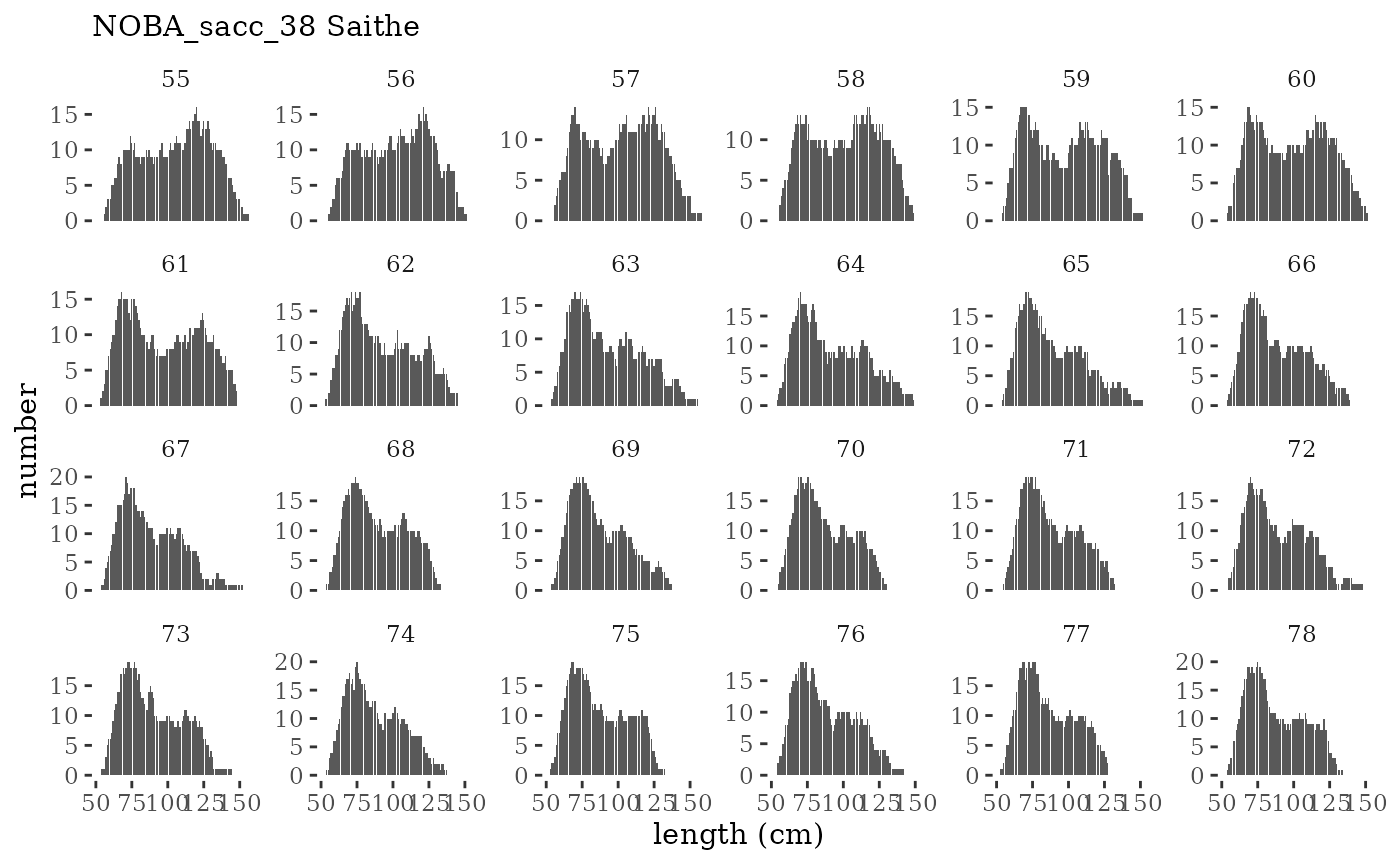
These plots represent the full mskeyrun simulated time series for the survey biomass index and weight at age, and a subset for length and age composition.

BTS_fall_allbox_effic1

BTS_spring_allbox_effic1

BTS_fall_allbox_effic1

BTS_spring_allbox_effic1

BTS_fall_allbox_effic1

BTS_spring_allbox_effic1

BTS_fall_allbox_effic1

BTS_spring_allbox_effic1

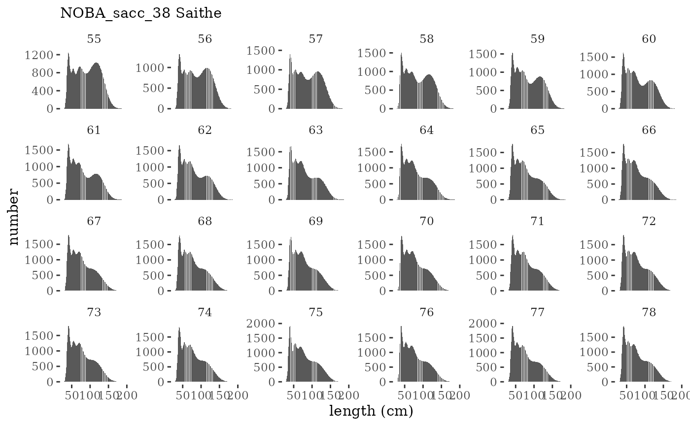
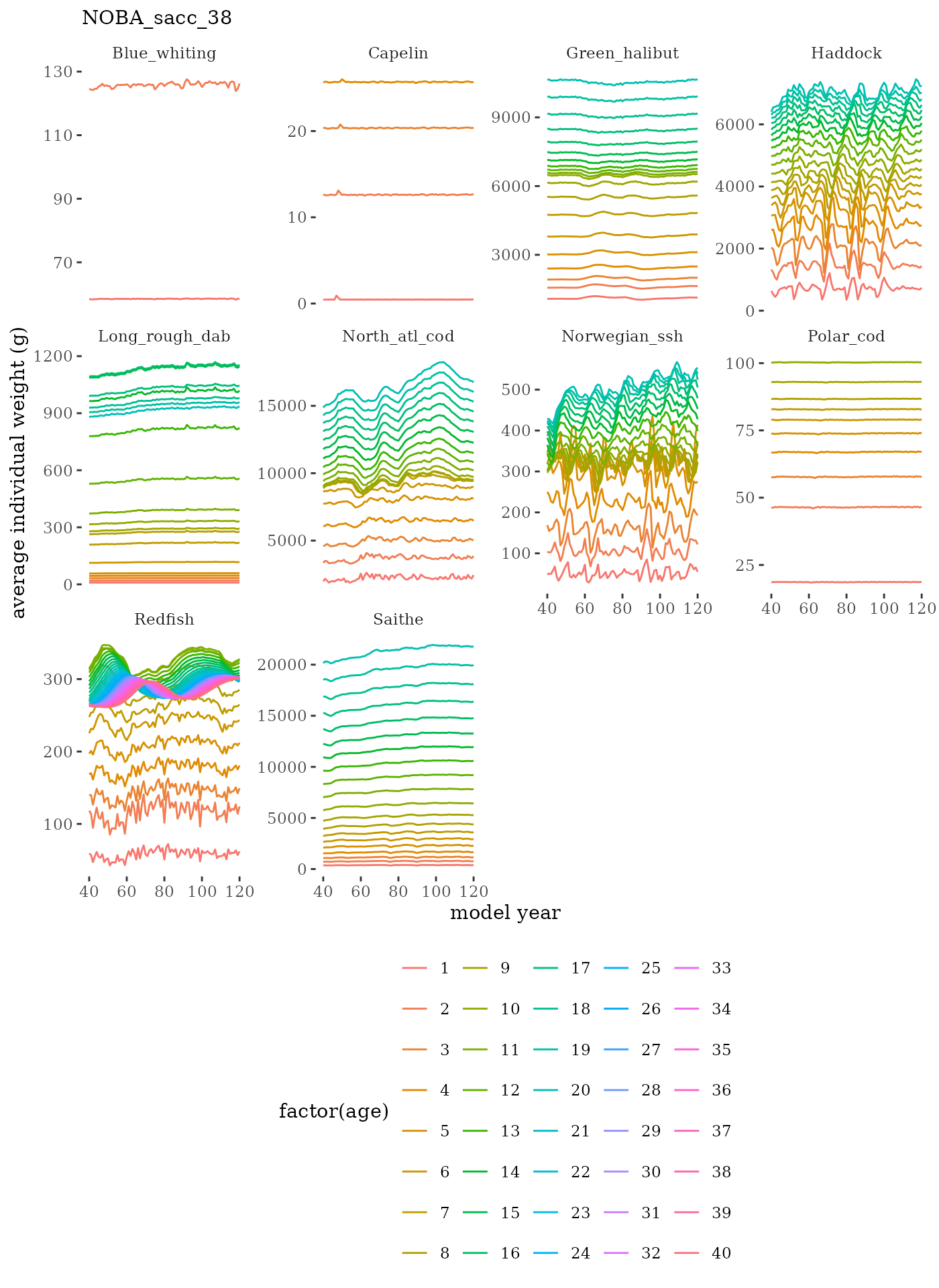
Visualize fishery data

These plots represent the the full mskeyrun simulated time series for fishery catch and weight at age, and a subset for length and age composition.

Write to model input files

Our goal was to have a reproducible process for all aspects of data generation through model inputs. The simulated data is included in the mskeyrun data package, data inputs are derived from those sources.

Multispecies surplus production model (MSSPM)

[To be added]

Length-structured multispecies model (Hydra)

Hydra input files were developed directly from mskeyrun datasets by modifying functions in the hydradata R package. The function create_Rdata_mskeyrun.R (code) allows the user to specify whether datasets should be constructed from Atlantis-simulated or real Georges Bank data, and the number of length bins to use for composition data, then creates an R data object. This data object is then used to create data and parameter input files using the function hydradata::create_datpin_files().

For example, this process creates the simulated dataset with 5 length bins:

The create_RData_mskeyrun.R file was sourced, and create_RData_mskeyrun("sim", nlenbin = 5) was run to make a new hydraDataList_msk.rda file in the package. Then the package is built locally, R is restarted, and the following code block is run to produce input files.

library(here)
library(hydradata)
inputs <- setup_default_inputs()
inputs$outDir <- here()

inputs$outputFilename <- "hydra_sim_NOBA_5bin_0comp" 

# tpl code removes 0 so replace in data
nbins <- hydraDataList_msk$Nsizebins
hydraDataList_msk$observedCatchSize[,7:(6+nbins)][hydraDataList_msk$observedCatchSize[,7:(6+nbins)]==0] <- 1e-4
hydraDataList_msk$observedSurvSize[,6:(5+nbins)][hydraDataList_msk$observedSurvSize[,6:(5+nbins)]==0] <- 1e-4

hydraDataList_5bin_0comp <- create_datpin_files(inputs,hydraDataList_msk)

# this saves the specific hydralist object, so we could saveRDS it to a diagnostics folder?
# advantage of rds format is we can assign it when reading it in to diagnostics scripts
saveRDS(hydraDataList_5bin_0comp, file.path(here("inputRdatalists/hydraDataList_5bin_0comp.rds")))

Run create_RData_mskeyrun("sim", nlenbin = 10) in hydradata, rebuild package, restart R, then…

library(here)
library(hydradata)
inputs <- setup_default_inputs()
inputs$outDir <- here()

inputs$outputFilename <- "hydra_sim_NOBA_10bin_0comp" 

# tpl code removes 0 so replace in data
nbins <- hydraDataList_msk$Nsizebins
hydraDataList_msk$observedCatchSize[,7:(6+nbins)][hydraDataList_msk$observedCatchSize[,7:(6+nbins)]==0] <- 1e-4
hydraDataList_msk$observedSurvSize[,6:(5+nbins)][hydraDataList_msk$observedSurvSize[,6:(5+nbins)]==0] <- 1e-4


hydraDataList_10bin_0comp <- create_datpin_files(inputs,hydraDataList_msk)

# this saves the specific hydralist object, so we could saveRDS it to a diagnostics folder?
# advantage of rds format is we can assign it when reading it in to diagnostics scripts
saveRDS(hydraDataList_10bin_0comp, file.path(here("inputRdatalists/hydraDataList_10bin_0comp.rds")))

Age structured multispecies statistical catch at age model (MSSCAA)

Work in progress here but not finished for October 2022 review.

References

Audzijonyte, A., Pethybridge, H., Porobic, J., Gorton, R., Kaplan, I., & Fulton, E. A. (2019). Atlantis: A spatially explicit end-to-end marine ecosystem model with dynamically integrated physics, ecology and socio-economic modules. Methods in Ecology and Evolution, 10(10), 1814–1819. https://doi.org/10.1111/2041-210X.13272

_eprint: https://besjournals.onlinelibrary.wiley.com/doi/pdf/10.1111/2041-210X.13272

Hansen, C., Drinkwater, K. F., Jähkel, A., Fulton, E. A., Gorton, R., & Skern-Mauritzen, M. (2019). Sensitivity of the Norwegian and Barents Sea Atlantis end-to-end ecosystem model to parameter perturbations of key species. PLOS ONE, 14(2), e0210419. https://doi.org/10.1371/journal.pone.0210419

Hansen, C., Skern-Mauritzen, M., Meeren, G. van der, Jähkel, A., & Drinkwater, K. F. (2016). Set-up of the Nordic and Barents Seas (NoBa) Atlantis model. Havforskningsinstituttet. https://imr.brage.unit.no/imr-xmlui/bitstream/handle/11250/2408609/FoH_2-2016.pdf?sequence=1&isAllowed=y

Sarah Gaichas

15 April, 2024

Simulating input data from an ecosystem model

Species in the ms-keyrun dataset

Generating a dataset

Configuration files specified once

Change these survey and fishery config files

Run atlantisom and save outputs

Create mskeyrun simulated data

Additional simulated data for food web models

Visualize simulated data

Plotting functions

Read in the “data” to check with plots

Visualize survey outputs

BTS_fall_allbox_effic1

BTS_spring_allbox_effic1

BTS_fall_allbox_effic1

BTS_spring_allbox_effic1

BTS_fall_allbox_effic1

BTS_spring_allbox_effic1

BTS_fall_allbox_effic1

BTS_spring_allbox_effic1

Visualize fishery data

Write to model input files

Multispecies surplus production model (MSSPM)

Length-structured multispecies model (Hydra)

Age structured multispecies statistical catch at age model (MSSCAA)

References