Calculating stratified mean biomass/abundance
Source:vignettes/calc_strat_mean.Rmd
calc_strat_mean.RmdBackground
The survdat package is designed to work with the
Northeast Fisheries Science Center’s (NEFSC) bottom trawl surveys. The
NEFSC has been conducting standardized bottom trawl surveys in the fall
since 1963 and spring since 1968. The surveys follow a stratified random
design. Fish species and several invertebrate species are enumerated on
a tow by tow basis [@Azarovitz_1981]. The
data are housed in the NEFSC’s survey database (SVDBS) maintained by the
Ecosystem Survey Branch.
The get_survdat_data function will query the NEFSC
survey database (SVSDBS) and apply the appropriate calibration factors
associated with gear or vessel differences throughout the time series.
However, end users are usually interested in more derived estimates of
biomass or abundance that the tow by tow data retrieved via
get_survdat_data. The stratified random design of the
survey allows for the calculation of a stratified mean biomass or
abundance for a species or group of species.
To facilitate the calculation of these stratified means, the
survdat package has the function
calc_stratified_mean. This function is actually a wrapper
of several intermediate functions.
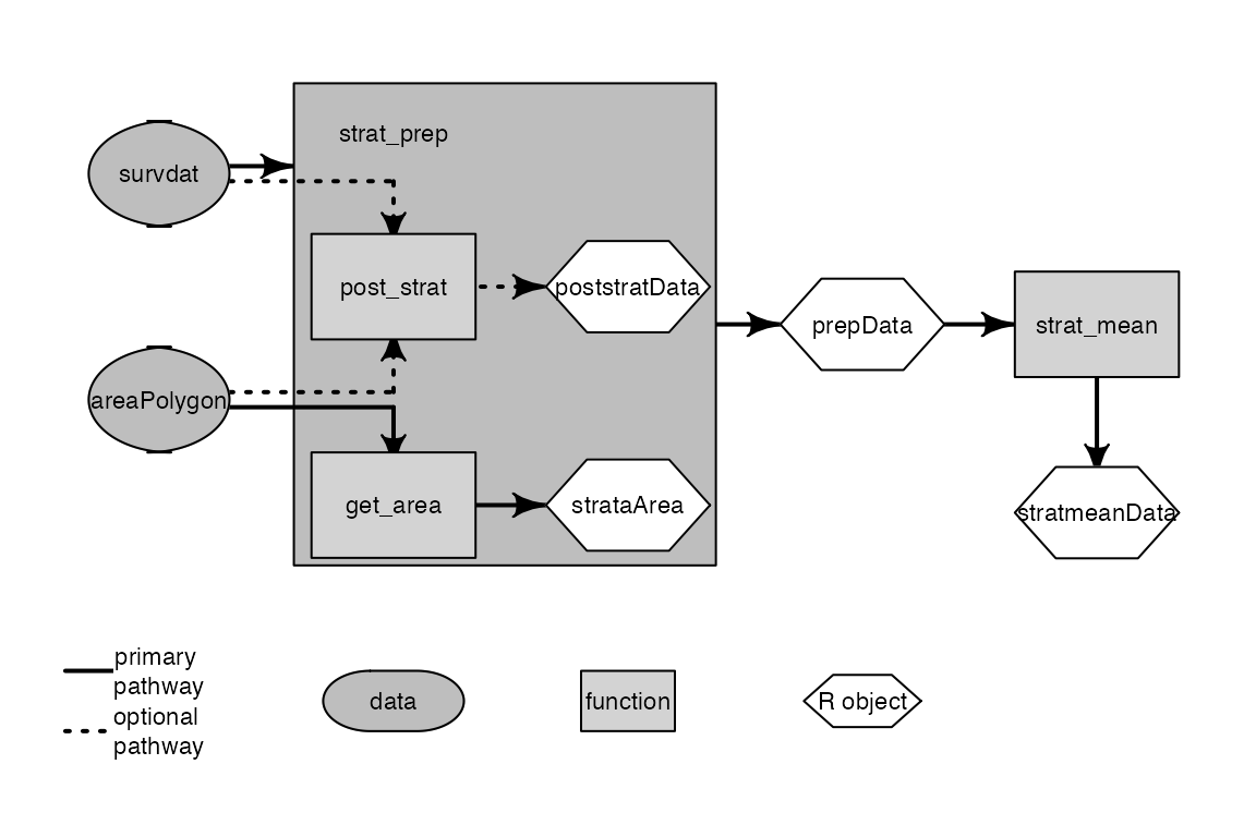
Work flow of the calc_stratified_mean function with
associated intermediate functions.
strat_prep
The first function called is strat_prep. As the name
implies, strat_prep prepares the data set so that the
stratified means can be calculated. Nested within this function are the
post_strat and get_area functions. The
post_strat function is used if not following the stratified
design of the survey. It is automatically called if the user inputs an
sf object rather than the specified default ‘NEFSC
strata’. When this occurs, the R object poststratData
generated by post_strat will replace the
survdat data object and is ultimately passed through to the
prepData object. This will also turn on the
poststratFlag which is used by the strat_mean
function.
At this point you can also filter the data using the
filterBySeason or filterByArea arguments. The
first will allow you to select one of three options: ‘FALL’,
‘SPRING’, or ‘all’. The default option is
‘all’. Note that selecting both the spring and fall survey will
combine the two surveys. So if you want to have separate means for both
surveys you need to run them independently. The second filter will allow
you to select a subset of strata to use in your analysis.
The rest of the prep work done by strat_prep is counting
the number of tows per strata and the proportional weight of the strata.
This adds the columns ntows and W.h to the
data set. The number of tows (ntows) is simply the length
of unique station records per stratum:
# Count the number of stations in each year for each Region
  data.table::setkey(stations, YEAR, STRAT)
  stations[, ntows := length(STATION), by = key(stations)]
Proportional weights of the strata are based on their area. The area
of the strata are calculated using the get_area function
which uses a Lambert Conformal Conic projection. The
get_area function creates a list of strata and their
corresponding areas (A) which strat_prep uses to calculate
the relative weight (W) of each strata h as:
After counting the number of tows and calculating the relative weight
of each strata, the resulting prepData is then passed to
the strat_mean function.
strat_mean
Once the data has been prepared using strat_prep the
real calculations are carried out in the function
strat_mean. This function will remove duplicate catch
records that may be present due to length data, merge sexed species (or
leave separate if specified), calculate the total number of stations for
the year, subset the species list if desired, and calculate the
stratified mean biomass and adundance along with the associated
variance.
The first few actions are straightforward. Length data is removed to ensure each catch is accounted for once.
#Remove length data if present
  data.table::setkey(stratmeanData, CRUISE6, STRATUM, STATION, SVSPP, CATCHSEX)
  stratmeanData <- unique(stratmeanData, by = key(stratmeanData))
  stratmeanData[, c('LENGTH', 'NUMLEN') := NULL]
Similarly, catch from sexed species such as spiny dogfish are merged
or kept separate. The default is to merge them but a user may specify to
keep them separate by setting the mergesexFlag to
FALSE. Sexed species are kept separate by changing their group
designation to a concatenation of their group name and catch sex.
#Merge sex or keep separate
  if(mergesexFlag == F) stratmeanData[, group := paste(group, CATCHSEX, sep = '')]

  data.table::setkey(stratmeanData, CRUISE6, strat, STATION, group)
  stratmeanData[, BIOMASS   := sum(BIOMASS),   by = key(stratmeanData)]
  stratmeanData[, ABUNDANCE := sum(ABUNDANCE), by = key(stratmeanData)]
  stratmeanData <- unique(stratmeanData, by = key(stratmeanData))
The total number of tows per year is the sum of ntows
for all of the strata sampled for a given year.
#Calculate total number of stations per year
  data.table::setkey(stratmeanData, strat, YEAR)
  N <- unique(stratmeanData, by = key(stratmeanData))
  N <- N[, sum(ntows), by = 'YEAR']
  data.table::setnames(N, 'V1', 'N')
Species or group list can be subsetted using the
filterByGroup argument.
Stratified mean and variance calculations
Finally, the stratified mean biomass is calculated as:
where is the stratified mean biomass, and the relative weight and mean biomass from stratum , and the total number of strata. is calculated as:
where is the biomass at station and the number of stations in stratum .
Additionally, variance is calculated as:
where is the variance of the stratified mean biomass and the variance of the mean for stratum . is calculated as:
If the poststratFlag was set to TRUE because a
different stratification was used rather than the survey design, the
variance calculation becomes:
where is the total number of stations for the year.
The final calculation for the calc_stratified_mean
function is the standard error of the mean which is:
Similar calculations are carried out for abundance with numbers replacing biomass in the equations above.
Tidy data
The default output from the calc_stratified_mean
function is a wide table with a row for every year/group combination.
You can elect a tidy format (long) instead by specifying the argument
tidy = TRUE. This will melt the table down so that
each year/group combo will now have a seperate row for stratified mean
biomass, stratified mean abundance, variance of the stratified mean
biomass, and variance of the stratified mean abundance. The tidy data
will also append a units column to the data set. The units for the
stratified mean biomass is
while the stratified mean abundance is
.
Note that the tidy data set does not include the standard errors.