Developing zooplankton indices in VAST

class: right, middle, my-title, title-slide

.title[
# Developing zooplankton indices in VAST
]
.subtitle[
## Herring Research Track <br /> 1 October 2024
]
.author[
### Sarah Gaichas, Adelle Molina
]

---

class: top, left

# Does food drive recruitment of Atlantic herring?

## Atlantic herring, *Clupea harengus*

.pull-left[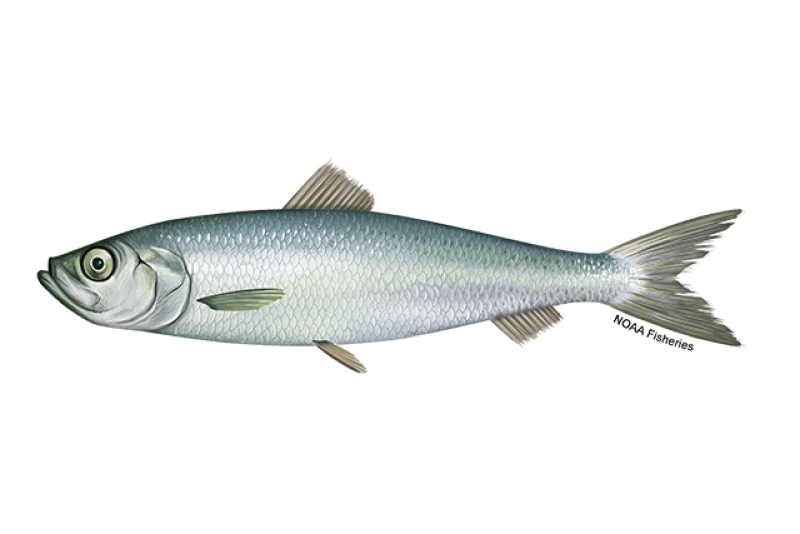
![Atlantic herring illustration, credit NOAA Fisheries](https://www.fisheries.noaa.gov/s3/styles/original/s3/2022-08/640x427-Herring-Atlantic-NOAAFisheries.png)
]

.pull-right[
.large[

"The herring is a plankton feeder.... Examination of 1,500 stomachs showed that adult herring near Eastport were living solely on copepods and on pelagic euphausiid shrimps (*Meganyctiphanes norwegica*), fish less than 4 inches long depending on the former alone, while the larger herring were eating both." <a name=cite-collette_bigelow_2002></a>([Collette et al., 2002](#bib-collette_bigelow_2002))

]
]

???
When first hatched, and before the disappearance of the yolk sac, the larvae (European) feed on larval snails and crustaceans, on diatoms, and on peridinians, but they soon begin taking copepods, and depend exclusively on these for a time after they get to be 12 mm. long, especially on the little Pseudocalanus elongatus. As they grow older they feed more and more on the larger copepods and amphipods, pelagic shrimps, and decapod crustacean larvae.

---
## Objective

Create zooplankton indices to evaluate changes in food for Atlantic herring larvae, juveniles, and adults over time and in space in the Northeast US continental shelf ecosystem.

Two applications:

1. Addressing uncertainty in the stock assessment for Atlantic herring (*Clupea harengus*)

1. Describing zooplankton species and group trends for integrated ecosystem assessment

.pull-left[
![Atlantic herring illustration, credit NOAA Fisheries](https://www.fisheries.noaa.gov/s3/styles/original/s3/2022-08/640x427-Herring-Atlantic-NOAAFisheries.png)
]

.pull-right[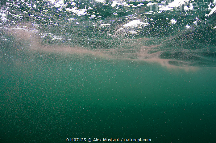
![copepods](https://nplimages.infradoxxs.com/cache/pcache2/01407135.jpg)
.footnote[
https://www.naturepl.com/stock-photo-copepods-calanus-finmarchicus-aggregated-at-the-surface-reverse-diel-nature-image01407135.html 
]
]

---
background-image: url("https://github.com/NOAA-EDAB/presentations/raw/master/docs/EDAB_images/AherringConceptualMod.png")
background-size: 1070px
background-position: bottom

## Which indicators are relevant for recruitment?

---
background-image: url("https://github.com/NOAA-EDAB/presentations/raw/master/docs/EDAB_images/AherringBRT_rec.png")
background-size: 800px
background-position: right

## Which indicators are relevant for recruitment?

.pull-left-30[
Boosted regression tree (Molina 2024) investigated relationships between environmental indicators and Atlantic herring recruitment estimated in the assessment.

Larval and juvenile food (zooplankton), egg predation, and temperature always highest influence
]

.pull-right-70[

]
---
## Northeast US [existing zooplankton indicators](https://noaa-edab.github.io/forageindex/ZooplanktonOverview.html)

.pull-left[
## Abundance anomalies in [`ecodata`](https://noaa-edab.github.io/ecodata/)

Ecosystem reporting areas: Ecosystem Production Units (EPUs) used for zooplankton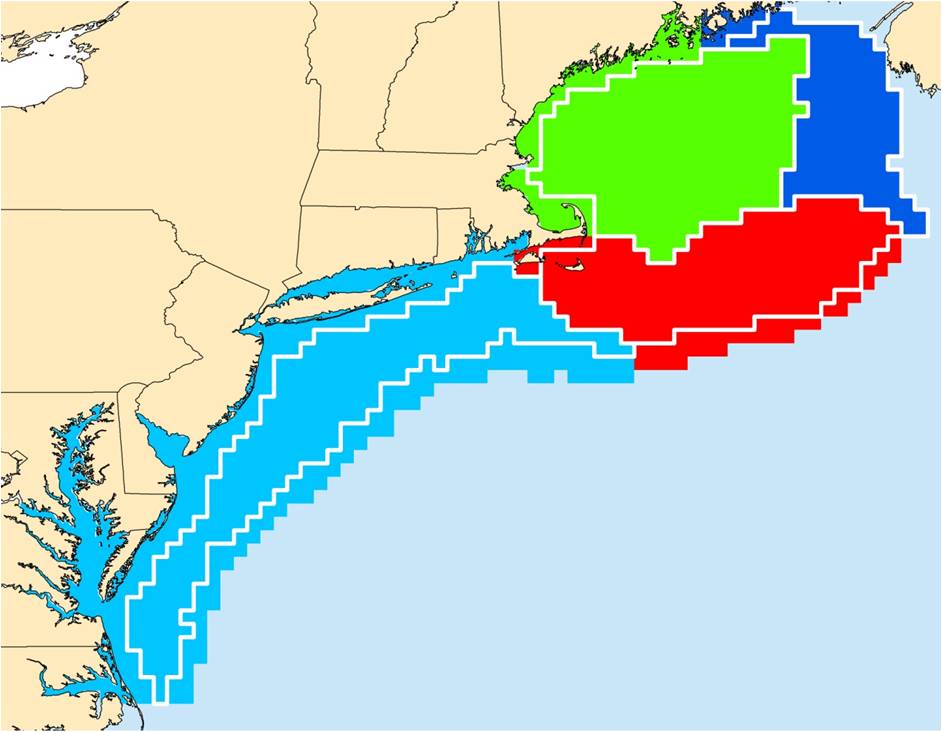

![EPU by ten minute squares](https://noaa-edab.github.io/tech-doc/images/EPUs.jpg)
]

.pull-right[

<img src="20241001_ZoopIndices_Gaichas_files/figure-html/unnamed-chunk-1-1.png" width="504" />
]

---
## Northeast US [existing zooplankton indicators](https://noaa-edab.github.io/forageindex/ZooplanktonOverview.html)

.pull-left[
## [Calanus stages](https://noaa-edab.github.io/tech-doc/calanus-stage.html), Gulf of Maine

]

.pull-right[

## *Calanus finmarchicus* time series by EPU

]
???

---
## Outline

.pull-left-60[

1. Vector Autoregressive Spatio-Temporal (VAST) modeling

1. Identify key zooplankton species: what are herring prey?

1. Which RE model is best? Selection

1. Spatial bounds for indices

1. Spatial and temporal bounds specific to herring larvae

1. Index trends

]

.pull-right-40[
![xkcd maps](https://imgs.xkcd.com/comics/heatmap.png)
.contrib[
https://xkcd.com/1138
]
]

---
## Vector Autoregressive Spatio-Temporal (VAST) modeling <a name=cite-thorson_comparing_2017></a><a name=cite-thorson_guidance_2019></a>([Thorson et al., 2017](https://doi.org/10.1093/icesjms/fsw193); [Thorson, 2019](http://www.sciencedirect.com/science/article/pii/S0165783618302820))

VAST is a Geostatistical generalized linear mixed effects model (GLMM) that models two linear predictors for an index: 1. encounter rate,  and 2. positive catch (amount in stomach)

A full model for the first linear predictor `$\rho_1$` for each observation `$i$` can include:
*  fixed intercepts `$\beta_1$` for each category `$c$` and time `$t$`, 
*  spatial random effects `$\omega_1$` for each location `$s$` and category, 
*  spatio-temporal random effects `$\varepsilon_1$` for each location, category, and time, 
*  fixed vessel effects `$\eta_1$` by vessel `$v$` and category, and 
*  fixed catchability impacts `$\lambda_1$` of covariates `$Q$` for each observation and variable `$k$`:

`$$\rho_1(i) = \beta_1(c_i, t_i) + \omega_1^*(s_i, c_i) + \varepsilon_1^*(s_i, c_i, t_i) + \eta_1(v_i, c_i) + \sum_{k=1}^{n_k} \lambda_1(k) Q(i,k)$$`

The full model for the second linear predictor `$\rho_2$` has the same structure, estimating `$\beta_2$`, `$\omega_2$`, `$\varepsilon_2$`, `$\eta_2$`, and `$\lambda_2$` using the observations, categories, locations, times, and covariates.

We modeled aggregate small pelagic prey as a single category, and apply a Poisson-link delta model to estimate expected prey mass per predator stomach as in <a name=cite-ng_predator_2021></a>([Ng et al., 2021](https://doi.org/10.1093/icesjms/fsab026)).

VAST model code and documentation: https://github.com/James-Thorson-NOAA/VAST

???
Spatial and spatio-temporal correlation decay with increasing distance estimated as `$\kappa$` in a Matern function with fixed smoothness and geometric anisotropy (directional correlation, optionally estimated by the model).

Initial model selection consistently supported the inclusion of spatial and spatio-temporal random effects and anisotropy across all datasets: fall, spring, and annual.

---
.pull-left-30[
## Spatial estimation assumptions

VAST has built-in "extrapolation grids" for many surveyed areas, including the Northeast US.

Observations in space are used to define fixed locations ("knots") covering the full extent of the model. We assume constant variation within a timestep at a knot.

Modelers specify the number of knots to group observation locations, to balance computation time and resolution. We used 500 knots:  
]

.pull-right-70[
![:img spring lgcopeALL knots, 90%](https://github.com/NOAA-EDAB/presentations/raw/master/docs/EDAB_images/Data_and_knots_lgcopeALL_spring.png)
]

???
Extrapolation grid: "area over which densities will be extrapolated to calculate derived quantities" encompassing survey area allows comparison with design-based estimates

Knots are defined that "minimize the average distance between samples and knots" using k-means clustering, which results in knots in proportion to sampling intensity across the area.

*THIS MEANS DIFFERENT DATASETS HAVE DIFFERENT GRIDS*

---
## Modeling spatial and spatio-temporal variation

.pull-left-60[
Observations correlated in space and in space over time due to unmeasured processes are modeled as multivariate normal Gaussian Random Fields (GRF):

`$\omega_1$` ~ MVN(0, `$\mathbf R_1$`); `$\omega_2$` ~ MVN(0, `$\mathbf R_2$`)   
`$\varepsilon_1$`(,t) ~ MVN(0, `$\mathbf R_1$`); `$\varepsilon_2$`(,t) ~ MVN(0, `$\mathbf R_2$`)

Spatial and spatio-temporal correlation decay with increasing distance `$\mathbf d$` estimated as `$\kappa$` in a Mat&eacute;rn function with fixed smoothness `$\nu$` and geometric anisotropy `$H$` (directional correlation). 
  
Correlation function between locations `$s$` and `$s'$`:

`$$\mathbf R_1(s, s') = \frac{1}{2^{\nu-1}\Gamma(\nu)} \times (\kappa_1 \lvert \mathbf d(s,s') \mathbf H  \rvert)^\nu \times K_\nu (\kappa_1 \lvert \mathbf d(s,s') \mathbf H  \rvert)$$`

Estimation uses stochastic partial differential equation (SPDE) approximation.

]

.pull-right-40[

![:img example spring lgcopeALL aniso, 85%](https://github.com/NOAA-EDAB/presentations/raw/master/docs/EDAB_images/Aniso_lgcopeALL_spring.png)

]

---
## Estimating density in space and the index

.pull-left[
Observation model "Index2", Gamma distribution for positive catches and Alternative "Poisson-link delta-model" using log-link for numbers-density and log-link for biomass per number. It is intended for continuous data, which includes biomass data and “numbers standardized to a fixed area.”

Probability of encounter Poisson: `$p(i) = 1 - exp[-n(i)]$` *set to 1 for groups found at all stations, e.g. small copepods or zooplankton volume*

Number of zooplankton cells per volume given encounter: `$r(i) = \frac{n(i)}{p(i)}w(i)$`

Probability for numbers per volume `$B$` where `$g$` is a Gamma function.  :

$$ Pr[b(i) = B] =  \begin{cases} 1-p(i), B = 0\\\\p(i) \times g[B|r(i), \sigma_b^2], B > 0 \end{cases},$$  
]

.pull-right[

Density `$b$` at a location (knot) `$s$` for year `$t$` is then the predicted number of cells per volume (linear predictor for encounter * linear predictor for cells/vol given encounter):

`$$\hat{b}_{s,t} = \hat{n}_{s,t}\hat{w}_{s,t}$$`

Index based on area `$a$` weighting for each of 500 knots (or subsets):

`$$I_t = \sum_{s=1}^{500} a_s\hat{b}_{s,t}$$`

Bias correction as in <a name=cite-thorson_implementing_2016></a>([Thorson et al., 2016](https://www.sciencedirect.com/science/article/pii/S0165783615301399))

]

???
I am interpreting zooplankton abundance per 100 cubic meters as numbers standardized to a fixed area (volume) in applying the Gamma observation model.

---
## Herring prey from adult stomachs: a mix of zooplankton

.pull-left-30[
![copepods](https://github.com/NOAA-EDAB/presentations/raw/master/IEA/HerringRT_2025/NOAAzooppics/pl23_fish7968.jpg)
![euphausiids](https://github.com/NOAA-EDAB/presentations/raw/master/IEA/HerringRT_2025/NOAAzooppics/pl23_fish3327.jpg)
.contrib[
Northeast Fisheries Science Center Diet Data Online: https://fwdp.shinyapps.io/tm2020/
]
]

.pull-right-70[

]

???

---
background-image: url("https://github.com/NOAA-EDAB/presentations/raw/master/docs/EDAB_images/AherringConceptualMod.png")
background-size: 600px
background-position: bottom

## Zooplankton groups

Focus is on recruitment, food for larvae through juveniles.

Models developed for the Herring RT are for the following copepod categories:

*   Large copepods ALL:  Calanus finmarchicus,  Metridia lucens, Calanus minor,  Eucalanus spp.,  Calanus spp.

*   Small copepods ALL:  Centropages typicus, Pseudocalanus spp., Temora longicornis, Centropages hamatus, Paracalanus parvus, Acartia spp., Clausocalanus arcuicornis, Acartia longiremis, Clausocalanus furcatus,  Temora stylifera, Temora spp., Tortanus discaudatus, Paracalanus spp.

???
*  Calanus finmarchicus (calfin_100m3) = "calfin" in table below,
*  Large copepods (calfin_100m3, mlucens_100m3, calminor_100m3, euc_100m3, calspp_100m3) = "lgcopeALL", 
*  Small copepods (all) (ctyp_100m3, pseudo_100m3, tlong_100m3, cham_100m3, para_100m3, acarspp_100m3, clauso, acarlong_100m3, fur_100m3, ost_100m3, temspp_100m3, tort_100m3, paraspp_100m3) = "smallcopeALL" and 
*  Small copepods (SOE) (ctyp_100m3, pseudo_100m3, tlong_100m3, cham_100m3) = "smallcopeSOE".

---
background-image: url("https://github.com/NOAA-EDAB/presentations/raw/master/docs/EDAB_images/Data_by_year_lgcopeALL_spring.png")
background-size: 600px
background-position: right top

## Sampling for zooplankton taxa

.pull-left[

Between 1982-2022 there were:

*  27774 NEFSC zooplankton survey stations.  
    +  52% between January-June (Spring). 
    +  48% between July-December (Fall).  
*  21524 with *Calanus finmarchicus*.  
    +  52% between January-June (Spring).   
    +  48% between July-December (Fall).  
*  23813 stations with large copepods. 
    +  49% between January-June (Spring).  
    +  51% between July-December (Fall).  
*  25255 stations with small copepods. 
    +  49% between January-June (Spring).  
    +  51% between July-December (Fall).  
*  11710 stations with euphausiids  
    +  50% between January-June (Spring).  
    +  50% between July-December (Fall). 
*  3815 stations with herring larvae
    +  28% between January-June (Spring).  
    +  72% between July-December (Fall).

]

.pull-right[

.center[
.footnote[
Zooplankton stations, January-June Northeast Fisheries Science Center surveys
]
]

]
???

---
## Model [selection](https://noaa-edab.github.io/zooplanktonindex/CopeModSelection.html)

Result: Always best to estimate spatial and spatio-temporal random effects

However, the small copepod fall model had the spatial random effects parameter for encounter rate,  `$\omega_1$`, approach 0. We allowed it to be estimated at 0 rather than fixing it at 0. Resulting indices were identical.

Only spring large zooplankton did better with a day of year catchability covariate

Did not have time to explore other catchability covariates or habitat covariates

Next steps might be to look at depth and or temperature

---
## Spatial partitioning: examining zooplankton trends at multiple scales

<div class="figure">
<img src="20241001_ZoopIndices_Gaichas_files/figure-html/maps-1.png" alt="Maps of key areas for Herring assessment indices. The full VAST model grid is shown in brown." width="33%" /><img src="20241001_ZoopIndices_Gaichas_files/figure-html/maps-2.png" alt="Maps of key areas for Herring assessment indices. The full VAST model grid is shown in brown." width="33%" /><img src="20241001_ZoopIndices_Gaichas_files/figure-html/maps-3.png" alt="Maps of key areas for Herring assessment indices. The full VAST model grid is shown in brown." width="33%" />
<p class="caption">Maps of key areas for Herring assessment indices. The full VAST model grid is shown in brown.</p>
</div>

Indices for zooplankton can be calculated for any subset of the full model domain. Bias correction of the resulting indices is then applied ([Thorson et al., 2016](https://www.sciencedirect.com/science/article/pii/S0165783615301399)).

???
NEFSC survey strata definitions are built into the VAST `northwest-atlantic` extrapolation grid already. We defined additional new strata to address the recreational inshore-offshore 3 mile boundary. The area within and outside 3 miles of shore was defined using the `sf` R package as a 3 nautical mile (approximated as 5.556 km) buffer from a high resolution coastline from the`rnaturalearth` R package. This buffer was then intersected with the current `FishStatsUtils::northwest_atlantic_grid` built into VAST and saved using code [here](https://github.com/sgaichas/bluefishdiet/blob/main/VASTcovariates_updatedPreds_sst_3mi.Rmd#L49-L94). Then, the new State and Federal waters strata were used to split NEFSC survey strata where applicable, and the new full set of strata were used along with a modified function from `FishStatsUtils::Prepare_NWA_Extrapolation_Data_Fn` to build a custom extrapolation grid for VAST as described in detail [here](https://sgaichas.github.io/bluefishdiet/VASTcovariates_finalmodbiascorrect_3misurvstrat.html).

---
background-image: url("https://github.com/NOAA-EDAB/presentations/raw/master/docs/EDAB_images/EPU_Designations_Map.jpg")
background-size: 450px
background-position: right

## Results: Compare ecodata and VAST annual *Calanus finmarchicus*

GB = Georges Bank, GOM = Gulf of Maine, MAB = Mid Atlantic Bight. Different calculation method, spatial definitions

---
background-image: url("https://github.com/NOAA-EDAB/presentations/raw/master/IEA/HerringRT_2025/mods/lgcopeALL_spring_500_biascorrect_doy/ln_density-predicted.png")
background-size: 560px
background-position: right top

## Results: Jan-Jun (Spring) large [copepods](https://noaa-edab.github.io/zooplanktonindex/CopeModResults.html)

.pull-left[

<img src="20241001_ZoopIndices_Gaichas_files/figure-html/lgcopespring-1.png" width="504" />
Model is bias corrected, includes a *day of year* "catchability" 
covariate which improved the fit.

]

.pull-right[
]
???

---
background-image: url("https://github.com/NOAA-EDAB/presentations/raw/master/IEA/HerringRT_2025/mods/smallcopeALL_fall_500_biascorrect/ln_density-predicted.png")
background-size: 560px
background-position: right top

## Results: Jul-Dec (Fall) small copepods

.pull-left[

<img src="20241001_ZoopIndices_Gaichas_files/figure-html/smcopefall-1.png" width="504" />
Model is bias corrected, does not include covariates.

]

.pull-right[
]
???

---
background-image: url("https://github.com/NOAA-EDAB/presentations/raw/master/IEA/HerringRT_2025/mods/herringlarvae_sepfeb_yrshift_500_biascorrect/ln_density-predicted.png")
background-size: 560px
background-position: right top

## When and where are [herring larvae](https://noaa-edab.github.io/zooplanktonindex/HerringLarvaeExplore.html) present?

.pull-left[

<img src="20241001_ZoopIndices_Gaichas_files/figure-html/herrlarvsepfeb-1.png" width="504" />
Herring larvae VAST model, timing for presence of larvae 
Sept. - Feb. <a name=cite-richardson_development_2010></a>([Richardson et al., 2010](https://doi.org/10.1093/icesjms/fsp276))

VAST estimated Fall forage biomass density &rarr;
]

.pull-right[
]
???
Based on herring larvae collected on the same surveys as the zooplankton
Year for January-February in this dataset was shifted to match September - December; this is the same cohort.

---
## Defining the larval herring area

.pull-left[
Herring larvae Sep-Feb VAST output:

*  Sum density by cell over all years
*  Evaluate quantiles of density in space
*  Select quantile with largest continuous area 
*  Outline "concave hull" of area
*  Integrate as new strata set into VAST grid
*  Run small copepods model with larval strata

*  27774 NEFSC zooplankton survey stations.  
    +  51% between September-February. 
    +  49% outside larval time.  
*  3815 stations with herring larvae
    +  93% between September-February. 
    +  7% outside larval time.  
*  25255 stations with small copepods. 
    +  52% between September-February. 
    +  48% outside larval time.

]

.pull-right[
<img src="20241001_ZoopIndices_Gaichas_files/figure-html/larvarea-1.png" width="504" />
]

---
background-image: url("https://github.com/NOAA-EDAB/presentations/raw/master/IEA/HerringRT_2025/mods/smallcopeALL_sepfeb_yrshift_500_larvarea_biascorrect/ln_density-predicted.png")
background-size: 560px
background-position: right top

## Small copepods available to larvae

.pull-left[

Model is bias corrected with no covariares.

]

.pull-right[
]
???

---
## Extensions: Other zooplankton indices could link to adult growth or survival (...next RTA)

.pull-left[
<img src="20241001_ZoopIndices_Gaichas_files/figure-html/zoovolspring-1.png" width="504" /><img src="20241001_ZoopIndices_Gaichas_files/figure-html/zoovolspring-2.png" width="504" />
]
.pull-right[
<img src="20241001_ZoopIndices_Gaichas_files/figure-html/unnamed-chunk-10-1.png" width="504" />

]

???
Potential risk criteria:

| Risk Level         | Definition                                                          |  
|:-------------------|:--------------------------------------------------------------------|
| Low  | Prey availability high (not limiting) and/or good fish condition past 5 years |
| Low-Moderate | Aggregate prey available for this species has stable or increasing trend, moderate condition |
| Moderate-High | Aggregate prey available for this species has significant decreasing trend, poor condition |
| High | Managed species highly dependent on prey with limited and declining availability, poor condition |

---
background-image: url("https://github.com/NOAA-EDAB/presentations/raw/master/docs/EDAB_images/SOE-MA-draft-03.16.23_Page_3.png")
background-size: 500px
background-position: right

## Next steps

These were implemented as recruitment covariates in WHAM

## Discussion

Further tailoring for herring?

These and other zooplankton indices will be submitted for

*  2025 ecosystem reporting

*  Time series for fitting or forcing food web models

*  Council risk indicators

Ideas for improvement welcome

---
## Thank you!  References

.contrib[
<a name=bib-collette_bigelow_2002></a>[Collette, B. B. et
al.](#cite-collette_bigelow_2002) (2002). _Bigelow and Schroeder's
Fishes of the Gulf of Maine, Third Edition_. 3rd ed. edition.
Washington, DC: Smithsonian Books. ISBN: 978-1-56098-951-6.

<a name=bib-ng_predator_2021></a>[Ng, E. L. et
al.](#cite-ng_predator_2021) (2021). "Predator stomach contents can
provide accurate indices of prey biomass". In: _ICES Journal of Marine
Science_ 78.3, pp. 1146-1159. ISSN: 1054-3139. DOI:
[10.1093/icesjms/fsab026](https://doi.org/10.1093%2Ficesjms%2Ffsab026).
URL:
[https://doi.org/10.1093/icesjms/fsab026](https://doi.org/10.1093/icesjms/fsab026)
(visited on Sep. 01, 2021).

<a name=bib-richardson_development_2010></a>[Richardson, D. E. et
al.](#cite-richardson_development_2010) (2010). "Development of
long-term larval indices for Atlantic herring (Clupea harengus) on the
northeast US continental shelf". In: _ICES Journal of Marine Science_
67.4, pp. 617-627. ISSN: 1054-3139. DOI:
[10.1093/icesjms/fsp276](https://doi.org/10.1093%2Ficesjms%2Ffsp276).
URL:
[https://doi.org/10.1093/icesjms/fsp276](https://doi.org/10.1093/icesjms/fsp276)
(visited on Aug. 30, 2024).

<a name=bib-thorson_guidance_2019></a>[Thorson, J.
T.](#cite-thorson_guidance_2019) (2019). "Guidance for decisions using
the Vector Autoregressive Spatio-Temporal (VAST) package in stock,
ecosystem, habitat and climate assessments". En. In: _Fisheries
Research_ 210, pp. 143-161. ISSN: 0165-7836. DOI:
[10.1016/j.fishres.2018.10.013](https://doi.org/10.1016%2Fj.fishres.2018.10.013).
URL:
[http://www.sciencedirect.com/science/article/pii/S0165783618302820](http://www.sciencedirect.com/science/article/pii/S0165783618302820)
(visited on Feb. 24, 2020).

<a name=bib-thorson_comparing_2017></a>[Thorson, J. T. et
al.](#cite-thorson_comparing_2017) (2017). "Comparing estimates of
abundance trends and distribution shifts using single- and multispecies
models of fishes and biogenic habitat". In: _ICES Journal of Marine
Science_ 74.5, pp. 1311-1321. ISSN: 1054-3139. DOI:
[10.1093/icesjms/fsw193](https://doi.org/10.1093%2Ficesjms%2Ffsw193).
URL:
[https://doi.org/10.1093/icesjms/fsw193](https://doi.org/10.1093/icesjms/fsw193)
(visited on Nov. 04, 2021).

<a name=bib-thorson_implementing_2016></a>[Thorson, J. T. et
al.](#cite-thorson_implementing_2016) (2016). "Implementing a generic
method for bias correction in statistical models using random effects,
with spatial and population dynamics examples". En. In: _Fisheries
Research_ 175, pp. 66-74. ISSN: 0165-7836. DOI:
[10.1016/j.fishres.2015.11.016](https://doi.org/10.1016%2Fj.fishres.2015.11.016).
URL:
[https://www.sciencedirect.com/science/article/pii/S0165783615301399](https://www.sciencedirect.com/science/article/pii/S0165783615301399)
(visited on Jul. 29, 2022).
]

.footnote[
Slides available at https://noaa-edab.github.io/presentations  
Contact: <Sarah.Gaichas@noaa.gov>
]