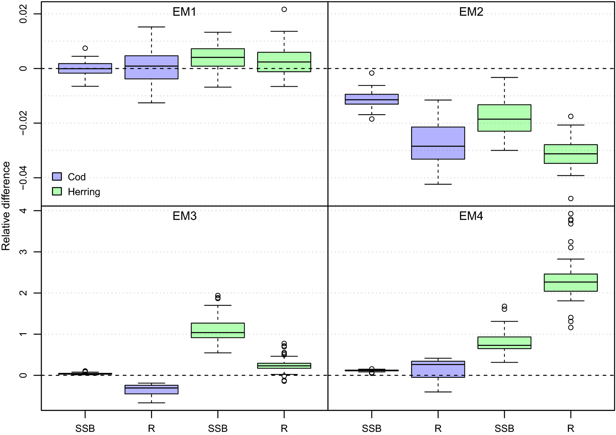
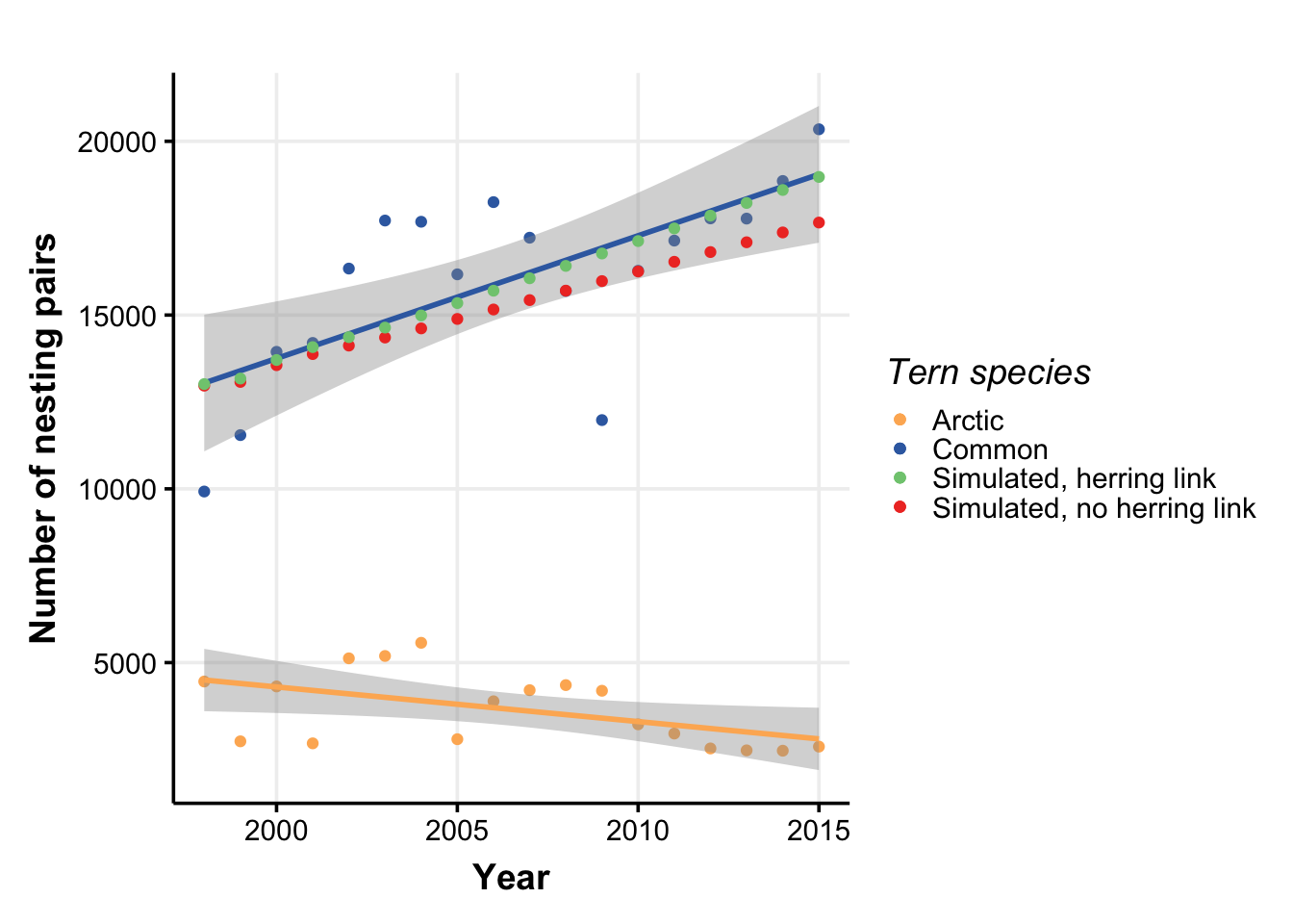
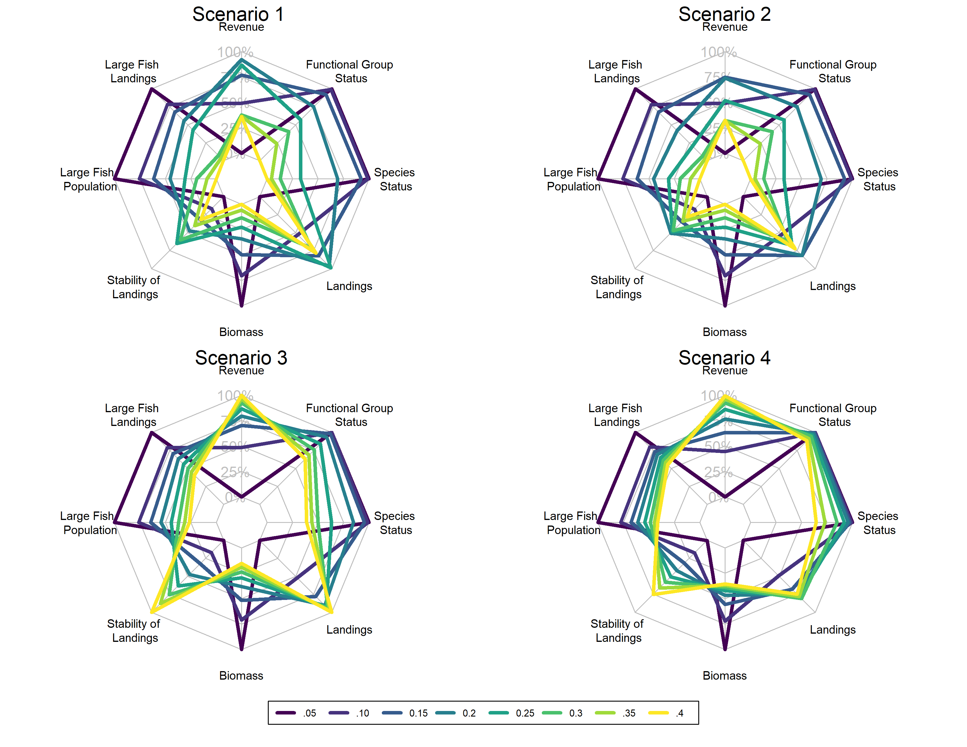
class: right, middle, my-title, title-slide # Species Interactions in Multispecies models ## NEFSC examples <br />NOAA FIT Workshop, 8 October 2020 ### Sarah Gaichas, Andy Beet, Kiersten Curti, Robert Gamble, and Sean Lucey <br /> Northeast Fisheries Science Center --- class: top, left background-image: url("EDAB_images/ecomods.png") background-size: contain ??? Alt text: Fisheries models range from single and multispecies models to full ecosystem models --- ## Why include species interactions? *Ignore predation at your peril: results from multispecies state-space modeling * <a name=cite-trijoulet_performance_2020></a>([Trijoulet, Fay, and Miller, 2020](https://besjournals.onlinelibrary.wiley.com/doi/abs/10.1111/1365-2664.13515)) >Ignoring trophic interactions that occur in marine ecosystems induces bias in stock assessment outputs and results in low model predictive ability with subsequently biased reference points. .pull-left-40[  EM1: multispecies state space EM2: multispecies, no process error EM3: single sp. state space, constant M EM4: single sp. state space, age-varying M *note difference in scale of bias for single species!* ] .pull-right-60[  ] ??? This is an important paper both because it demonstrates the importance of addressing strong species interactions, and it shows that measures of fit do not indicate good model predictive performance. Ignoring process error caused bias, but much smaller than ignoring species interactions. See also Vanessa's earlier paper evaluating diet data interactions with multispecies models --- background-image: url("EDAB_images/modeling_study.png") background-size: 380px background-position: right bottom # Today: compare and contrast species interactions ## Multispecies catch at age <a name=cite-curti_evaluating_2013></a>([Curti, Collie, Legault, and Link, 2013](http://www.nrcresearchpress.com/doi/abs/10.1139/cjfas-2012-0229)) ## Multispecies catch at length <a name=cite-gaichas_combining_2017></a>([Gaichas, Fogarty, Fay, Gamble, Lucey, and Smith, 2017](https://academic.oup.com/icesjms/article/74/2/552/2669545/Combining-stock-multispecies-and-ecosystem-level)) ## Multispecies production <a name=cite-gamble_analyzing_2009></a>([Gamble and Link, 2009](http://linkinghub.elsevier.com/retrieve/pii/S0304380009003998)) ## Food web <a name=cite-lucey_conducting_2020></a>([Lucey, Gaichas, and Aydin, 2020](http://www.sciencedirect.com/science/article/pii/S0304380020301290)) ## MICE for MSE <a name=cite-deroba_dream_2018></a>([Deroba, Gaichas, Lee, Feeney, Boelke, and Irwin, 2018](http://www.nrcresearchpress.com/doi/10.1139/cjfas-2018-0128)) --- ## Multispecies catch at age estimation model: *seeking catchy name* [FIT: MSCAA](https://nmfs-ecosystem-tools.github.io/MSCAA/) Species interactions: - Predation: Top down only (predators increase M of prey, predators grow regardless of prey) *Based on standard age structured stock assessment population dynamics equations* - First, split `\(M\)` for species `\(i\)` age `\(a\)` into components: `$$M_{i,a,t} = M1_i + M2_{i,a,t}$$` - Calculate `\(M2\)` with MSVPA predation equation, which applies a predator consumption:biomass ratio to the suitable prey biomass for that predator. - Suitability is a function of predator size preference (based on an age-specific predator:prey weight ratio) and prey vulnerability (everything about the prey that isn't size related). - Also sensitive to "other food" `$$M2_{i,a,t} = \frac{1}{N_{i,a,t}W_{i,a,t}}\sum_j \sum_b CB_{j,b} B_{j,b,t} \frac{\phi_{i,a,j,b,t}}{\phi_{j,b,t}}$$` ??? Size preference is `$$g_{i,a,j,b,t}=\exp\bigg[\frac{-1}{2\sigma_{i,j}^2}\bigg(\ln\frac{W_{j,b,t}}{W_{i,a,t}}-\eta_{i,j}\bigg)^2\bigg]$$` Suitability, `\(\nu\)` of prey `\(i\)` to predator `\(j\)`: `$$\nu_{i,a,j,b,t}=\rho_{i,j}g_{i,a,j,b,t}$$` Scaled suitability: `$$\tilde\nu_{i,a,j,b,t}=\frac{\nu_{i,a,j,b,t}}{\sum_i \sum_a \nu_{i,a,j,b,t} + \nu_{other}}$$` Suitable biomass of prey `\(i\)` to predator `\(j\)`: `$$\phi_{i,a,j,b,t}=\tilde\nu_{i,a,j,b,t}B_{i,a,t}$$` Available biomass of other food, where `\(B_other\)` is system biomass minus modeled species biomass: `$$\phi_{other}=\tilde\nu_{other}B_{other,t}$$` Total available prey biomass: `$$\phi_{j,b,t}=\phi_{other} + \sum_i \sum_a \phi_{i,a,j,b,t}$$` --- ## Multispecies catch at length simulation model: [Hydra](https://github.com/NOAA-EDAB/hydra_sim) Species interactions: - Predation: Top down only (predators increase M of prey, predators grow regardless of prey) *Same MSVPA predation equation as MSCAA (but length based), same dependencies and caveats* - Suitability, `\(\rho\)`, of prey species `\(m\)` size `\(n\)` for a given predator species `\(i\)` size `\(j\)` a function of size preference and vulnerability {0,1}. - Food intake `\(I\)` for each predator-at-size is temperature dependent consumption rate times mean stomach content weight. `$$M2_{m,n,t} = \sum_i \sum_j I_{i,j,t} N_{i,j,t} \frac{\rho_{i,j,m,n}}{\sum_a \sum_b \rho_{i,j,a,b} W_{a,b} N_{a,b} + \Omega}$$` *Associated GitHub repositories* * [hydra-sim Wiki](https://github.com/NOAA-EDAB/hydra_sim/wiki) * [hydradata](https://github.com/NOAA-EDAB/hydradata) * [LeMANS](https://github.com/NOAA-EDAB/LeMANS) * [hydra-est](https://github.com/NOAA-EDAB/hydra_est) Work in progress to convert to estimation model * [mscatch](https://github.com/NOAA-EDAB/mscatch) Multispecies fishery catch data ??? But: - Covariates on growth, maturity, recruitment possible; intended for environmental variables - So could hack in prey-dependent growth but making it dynamic is difficult We specify 'preferred' predator-prey weight ratio (log scale) `\(\Psi_j\)` and variance in predator size preference `\(\sigma_j\)` to compare with the actual predator-prey weight ratio `\((w_n / w_j)\)` to get the size preference `\(\vartheta\)`. `$$\vartheta_{n,j} = \frac{1}{(w_n / w_j)\sigma_j \sqrt{2\pi}} e^{-\frac{[log_e(w_n / w_j) - \Psi_j]}{2\sigma_j^2}}$$` Food intake is `$$I_{i,j,t} = 24 [\delta_j e^{\omega_i T}]\bar{C}_{i,j,k,t}$$` --- ## Multispecies production simulation: [Kraken](https://github.com/NOAA-EDAB/Kraken) and estimation [FIT: MSSPM](https://nmfs-ecosystem-tools.github.io/MSSPM/) Species interactions: - Predation: Top down (predation decreases population growth of prey, predator population growth independent of prey) - Competition: Within and between species groups *Based on Shaefer and Lotka-Volterra population dynamics and predation equations* - Species have intrinsic population growth rate `\(r_i\)` - Full model has - Carrying capacity `\(K\)` at the species group level `\(K_G\)` and at the full system level `\(K_\sigma\)` - Within group competition `\(\beta_{ig}\)` and between group competition `\(\beta_{iG}\)` slow population growth near `\(K\)` - Predation `\(\alpha_{ip}\)` and harvest `\(H_i\)` reduce population `$$\frac{dN_i}{dt} = r_iN_i \bigg(1 - \frac{N_i}{K_G} - \frac{\sum_g \beta_{ig}N_g}{K_G} - \frac{\sum_G \beta_{iG}N_G}{K_\sigma - K_G} \bigg) - N_i\sum_p\alpha_{ip}N_p - H_iN_i$$` - Simpler version used in most applications has interaction coefficient `\(\alpha\)` that incorporates carrying capacity `$$B_{i,t+1}=B_{i,t} + r_iB_{i,t} - B_{i,t}\sum_j\alpha_{i,j}B_{j,t} - C_{i,t}$$` ??? Interaction coefficients `\(\alpha_{i,j}\)` can be positive or negative `\(C\)` can be a Catch time series, an exploitation rate time series `\(B_{i,t}*F_{i,t}\)` or an `\(qE\)` (catchability/Effort) time series. Environmental covariates can be included on growth or carrying capacity (in the model forms that have an explicit carrying capacity). --- background-image: url("EDAB_images/Balance_concept.png") background-size: 700px background-position: right ## Food web: [Rpath](https://github.com/NOAA-EDAB/Rpath) in collaboration with AFSC .pull-left[ Species interactions: - Full predator-prey: Consumption leads to prey mortality and predator growth - Static and dynamic model components Static model: For each group, `\(i\)`, specify: Biomass `\(B\)` (or Ecotrophic Efficiency `\(EE\)`) Population growth rate `\(\frac{P}{B}\)` Consumption rate `\(\frac{Q}{B}\)` Diet composition `\(DC\)` Fishery catch `\(C\)` Biomass accumulation `\(BA\)` Im/emigration `\(IM\)` and `\(EM\)` Solving for `\(EE\)` (or `\(B\)`) for each group: `$$B_i\Big(\frac{P}{B}\Big)_i*EE_i+IM_i+BA_i=\sum_{j}\Big[ B_j\Big (\frac{Q}{B}\Big)_j*DC_{ij}\Big ]+EM_i+C_i$$` ] .pull-right[ ] ??? Predation mortality `$$M2_{ij} = \frac{DC_{ij}QB_jB_j}{B_i}$$` Fishing mortality `$$F_i = \frac{\sum_{g = 1}^n (C_{ig,land} + C_{ig,disc})}{B_i}$$` Other mortality `$$M0_i = PB_i \left( 1 - EE_i \right)$$` --- background-image: url("EDAB_images/ForagingArena.png") background-size: 380px background-position: right ## Food web: [Rpath](https://github.com/NOAA-EDAB/Rpath) in collaboration with AFSC .pull-left-70[ Dynamic model (with MSE capability): `$$\frac{dB_i}{dt} = \left(1 - A_i - U_i \right) \sum_{j} Q \left(B_i, B_j \right) - \sum_{j} Q \left( B_j, B_i \right) - M0_iB_i - C_m B_i$$` Consumption: `$$Q \left( B_i, B_j \right) = Q_{ij}^* \Bigg( \frac{V_{ij} Ypred_j}{V_{ij} - 1 + \left( 1 - S_{ij} \right) Ypred_j + S_{i} \sum_k \left( \alpha_{kj} Ypred_k \right)} \Bigg) \times \\\Bigg( \frac{D_{ij} Yprey_i^{\theta_{ij}}}{D_{ij} - 1 + \big( \left( 1 - H_{ij} \right) Yprey_i + H_{i} \sum_k \left( \beta_{ik} Yprey_k \right) \big)^{\theta_{ij}}} \Bigg)$$` Where `\(V_{ij}\)` is vulnerability, `\(D_{ij}\)` is “handling time” accounting for predator saturation, and `\(Y\)` is relative biomass which may be modified by a foraging time multiplier `\(Ftime\)`, `$$Y[pred|prey]_j = Ftime_j \frac {B_j}{B_j^*}$$` ] .pull-right-30[ ] ??? The parameters `\(S_{ij}\)` and `\(H_{ij}\)` are flags that control whether the predator density dependence `\(S_{ij}\)` or prey density dependence `\(H_{ij}\)` are affected solely by the biomass levels of the particular predator and prey, or whether a suite of other species’ biomasses in similar roles impact the relationship. For the default value for `\(S_{ij}\)` of 0 (off), the predator density dependence is only a function of that predator biomass and likewise for prey with the default value of 0 for `\(H_{ij}\)`. Values greater than 0 allow for a density-dependent effects to be affected by a weighted sum across all species for predators, and for prey. The weights `\(\alpha_{kj}\)` and `\(\beta_{kj}\)` are normalized such that the sum for each functional response (i.e. `\(\sum_k\alpha_{kj}\)` and `\(\sum_k\beta_{kj}\)` for the functional response between predator *j* and prey *i*) sum to 1. The weights are calculated from the density-independent search rates for each predator/prey pair, which is equal to `\(2Q_{ij}^*V_{ij} / (V_{ij} - 1)B_i^*B_j^*\)`. --- background-image: url("EDAB_images/OMdesign.png") background-size: 750px background-position: right ## MICE for MSE: Linked models .pull-left-30[ *Develop a harvest control rule considering herring's role as prey* Species interactions: - Bottom up only: Predators with herring dependent dynamics - NO predator feedback to herring - Alternative Herring operating models with high and low M (Also, done in ~ 6 months) ] .pull-right-70[] --- background-image: url("EDAB_images/herrtopreds.png") background-size: 640px background-position: left ## MICE for MSE Predators: deterministic delay-difference population models with herring-predator links .pull-left[] .pull-right[.right[  ] .table[ Time constraints forced: - selection of predators with previous modeling and readily available data - selection of single strongest herring-predator relationship - models ignoring high variance in prey-predator relationships ] ] ??? In general, if support for a relationship between herring and predator recruitment was evident, it was modeled as a predator recruitment multiplier based on the herring population `\(N_{y}\)` relative to a specified threshold `\(N_{thresh}\)`: `$$\bar{R}_{y+a}^P = R_{y+a}^P * \frac{\gamma(N_{y}/N_{thresh})}{(\gamma-1)+(N_{y}/N_{thresh})}$$` where `\(\gamma\)` > 1 links herring population size relative to the threshold level to predator recruitment. If a relationship between predator growth and herring population size was evident, annual changes in growth were modeled by modifying either the Ford-Walford intercept `\(\alpha_y^P\)` or slope `\(\rho_y^P\)`: `$$B_{y+1}^P = S_{y}^P (\alpha_y^P N_{y}^P + Fw_{slope} B_{y}^P) + \alpha_y^PR_{y+1}^P$$` or `$$B_{y+1}^P = S_{y}^P (Fw_{int} N_{y}^P + \rho_y^P B_{y}^P) + Fw_{int} R_{y+1}^P$$` where either `\(\alpha_y^P\)` or `\(\rho_y^P\)` are defined for a predator using herring population parameters. Finally, herring population size `\(N_{y}\)` could be related to predator survival using an annual multiplier on constant predator annual natural mortality `\(v\)`: `$$v_{y} = v e ^ {-(\frac{N_{y}}{N_{F=0}})\delta}$$` where 0 < `\(\delta\)` <1 links herring population size to predator survival. --- background-image: url("EDAB_images/herrup10pann.png") background-size: 830px background-position: right bottom ## Epilogue: Herring MSE food web modeling supplemental results - Tradeoffs between forage groups and mixed impacts to predators apparent when multiple species and full predator prey interaction feedbacks can be included .pull-left-30[ - Rpath Ecosense functions evaluate parameter uncertainty within a scenario - Now we have MSE closed loop possibilities in Rpath! - Can implement HCRs with predator prey interactions (Lucey et al. accepted) ] .pull-right-70[ ] --- ## References .contrib[ <a name=bib-curti_evaluating_2013></a>[Curti, K. L, J. S. Collie, C. M. Legault, et al.](#cite-curti_evaluating_2013) (2013). "Evaluating the performance of a multispecies statistical catch-at-age model". En. In: _Canadian Journal of Fisheries and Aquatic Sciences_ 70.3, pp. 470-484. ISSN: 0706-652X, 1205-7533. DOI: [10.1139/cjfas-2012-0229](https://doi.org/10.1139%2Fcjfas-2012-0229). URL: [http://www.nrcresearchpress.com/doi/abs/10.1139/cjfas-2012-0229](http://www.nrcresearchpress.com/doi/abs/10.1139/cjfas-2012-0229) (visited on Jan. 13, 2016). <a name=bib-deroba_dream_2018></a>[Deroba, J. J, S. K. Gaichas, M. Lee, et al.](#cite-deroba_dream_2018) (2018). "The dream and the reality: meeting decision-making time frames while incorporating ecosystem and economic models into management strategy evaluation". In: _Canadian Journal of Fisheries and Aquatic Sciences_. ISSN: 0706-652X. DOI: [10.1139/cjfas-2018-0128](https://doi.org/10.1139%2Fcjfas-2018-0128). URL: [http://www.nrcresearchpress.com/doi/10.1139/cjfas-2018-0128](http://www.nrcresearchpress.com/doi/10.1139/cjfas-2018-0128) (visited on Jul. 20, 2018). <a name=bib-gaichas_combining_2017></a>[Gaichas, S. K, M. Fogarty, G. Fay, et al.](#cite-gaichas_combining_2017) (2017). "Combining stock, multispecies, and ecosystem level fishery objectives within an operational management procedure: simulations to start the conversation". In: _ICES Journal of Marine Science_ 74.2, pp. 552-565. ISSN: 1054-3139. DOI: [10.1093/icesjms/fsw119](https://doi.org/10.1093%2Ficesjms%2Ffsw119). URL: [https://academic.oup.com/icesjms/article/74/2/552/2669545/Combining-stock-multispecies-and-ecosystem-level](https://academic.oup.com/icesjms/article/74/2/552/2669545/Combining-stock-multispecies-and-ecosystem-level) (visited on Oct. 18, 2017). <a name=bib-gamble_analyzing_2009></a>[Gamble, R. J. and J. S. Link](#cite-gamble_analyzing_2009) (2009). "Analyzing the tradeoffs among ecological and fishing effects on an example fish community: A multispecies (fisheries) production model". En. In: _Ecological Modelling_ 220.19, pp. 2570-2582. ISSN: 03043800. DOI: [10.1016/j.ecolmodel.2009.06.022](https://doi.org/10.1016%2Fj.ecolmodel.2009.06.022). URL: [http://linkinghub.elsevier.com/retrieve/pii/S0304380009003998](http://linkinghub.elsevier.com/retrieve/pii/S0304380009003998) (visited on Oct. 13, 2016). <a name=bib-lucey_conducting_2020></a>[Lucey, S. M, S. K. Gaichas, and K. Y. Aydin](#cite-lucey_conducting_2020) (2020). "Conducting reproducible ecosystem modeling using the open source mass balance model Rpath". En. In: _Ecological Modelling_ 427, p. 109057. ISSN: 0304-3800. DOI: [10.1016/j.ecolmodel.2020.109057](https://doi.org/10.1016%2Fj.ecolmodel.2020.109057). URL: [http://www.sciencedirect.com/science/article/pii/S0304380020301290](http://www.sciencedirect.com/science/article/pii/S0304380020301290) (visited on Apr. 27, 2020). <a name=bib-trijoulet_performance_2020></a>[Trijoulet, V, G. Fay, and T. J. Miller](#cite-trijoulet_performance_2020) (2020). "Performance of a state-space multispecies model: What are the consequences of ignoring predation and process errors in stock assessments?" En. In: _Journal of Applied Ecology_ n/a.n/a. ISSN: 1365-2664. DOI: [10.1111/1365-2664.13515](https://doi.org/10.1111%2F1365-2664.13515). URL: [https://besjournals.onlinelibrary.wiley.com/doi/abs/10.1111/1365-2664.13515](https://besjournals.onlinelibrary.wiley.com/doi/abs/10.1111/1365-2664.13515) (visited on Dec. 04, 2019). ] ## Additional resources * [New England herring MSE peer review](https://s3.amazonaws.com/nefmc.org/Final-Peer-review-report.pdf) * [New England herring MSE debrief](https://s3.amazonaws.com/nefmc.org/3_Herring-MSE-debrief-final-report.pdf) .footnote[ Slides available at https://noaa-edab.github.io/presentations Contact: <Sarah.Gaichas@noaa.gov> ] --- --- ## Hydra: details and current uses .pull-left[ *2018 CIE for Ecosystem Based Fishery Management Strategy* * [EBFM strategy review](https://www.nefsc.noaa.gov/program_review/) * Multispecies model simulations <img src="EDAB_images/EBFM HCR.png" width="75%" /> ] .pull-right[  ] --- ## Herring MSE details: Operating models and uncertainties .pull-left-70[ .table[ |Operating Model Name|Herring Productivity|Herring Growth|Assessment Bias| |:---------------------|:---------------------|:-----------------|:-----------------| | LowFastBiased | Low: high M, low h (0.44) | 1976-1985: fast | 60% overestimate | | LowSlowBiased | Low: high M, low h (0.44) | 2005-2014: slow | 60% overestimate | | LowFastCorrect | Low: high M, low h (0.44) | 1976-1985: fast | None | | LowSlowCorrect | Low: high M, low h (0.44) | 2005-2014: slow | None | | HighFastBiased | High: low M, high h (0.79) | 1976-1985: fast | 60% overestimate | | HighSlowBiased | High: low M, high h (0.79) | 2005-2014: slow | 60% overestimate | | HighFastCorrect | High: low M, high h (0.79) | 1976-1985: fast | None | | HighSlowCorrect | High: low M, high h (0.79) | 2005-2014: slow | None | ] &nbsp; &nbsp; ] .pull-right-30[ ([Deroba, Gaichas, Lee, et al., 2018](http://www.nrcresearchpress.com/doi/10.1139/cjfas-2018-0128)) ] Implementation error was included as year-specific lognormal random deviations: `\(F_{a,y}=\bar{F}_yS_ae^{\varepsilon_{\theta,y}-\frac{\sigma_\theta^2}{2}} \;\;\; \varepsilon_{\theta} \sim N(0,\sigma_\theta^2)\)` Assessment error was modeled similarly, with first-order autocorrelation and an optional bias term `\(\rho\)`: `\(\widehat{N}_{a,y}=[N_{a,y}(\rho+1)]e^{\varepsilon_{\phi,y}-\frac{\sigma_\phi^2}{2}}\;\;\;\; \varepsilon_{\phi,y}=\vartheta\varepsilon_{\phi,y-1}+\sqrt{1-\vartheta^2}\tau_y \;\;\;\; \tau \sim N(0,\sigma_\phi^2)\)` --- background-image: url("EDAB_images/herrtopreds_results.png") background-size: 650px background-position: left center ## Herring MSE details: Results summary Three HCR types were rejected at the second stakeholder meeting for poor fishery and predator performance. .pull-left[] .pull-right[.right[ <img src="20201008_FIT_MSmods_Gaichas_files/figure-html/ZZZ-1.png" width="80%" /> ]] --- ## Managing tradeoffs under uncertainty: What control rules give us 90% of everything we want? - Tern productivity at 1.0 or above more than 90% of the time - Herring biomass more than 90% of SSBmsy - Fishery yield more than 90% of MSY &nbsp; - AND fishery closures (F=0) less than 1% of the time (plot on right). .pull-left[ <img src="20201008_FIT_MSmods_Gaichas_files/figure-html/unnamed-chunk-2-1.png" width="504" /> ] .pull-right[ <img src="20201008_FIT_MSmods_Gaichas_files/figure-html/unnamed-chunk-3-1.png" width="504" /> ]