Ecosystem Context for Stock Advice: Northern component of the black sea bass stock

1 Introduction

This report provides contextual ecosystem information for northern component of the black sea bass (Centropristis striata) stock on the Northeast U.S. Continental Shelf. Data extractions for spring and fall are confined to the black sea bass stock area based on respective survey strata sets. The information is intended to span a range of potential factors affecting the productivity and distribution of black sea bass, including: surface and bottom temperature and salinity, chlorophyll concentration, indices of habitat, diet composition, and abundance of key zooplankton prey of larval black sea bass. These factors can be used to qualitatively inform the interpretation of population status and/or quantitatively improve model responsiveness to ecosystem factors. The range and complexity of ecosystem data makes it unlikely to find the most relevant and comprehensive factor variables with a first evaluation; this process will require an iterative approach of evaluation and feedback. Additional indices can be included to address the needs of the working group.

Summary

The thermal environment for the northern component of the black sea bass stock during spring has not changed significantly with the only perceivable trend seen in the bottom temperature associated with the southern end or component of the stock. However, there is stronger evidence of environmental change with both salinity and chlorophyll concentration, with salinity increasing and chlorophyll decreasing. It should be kept in mind that the stronger signals of thermal change are associated with summer and fall conditions on the NE Shelf. The area of spring occupancy habitat has increased for black sea bass, with the most dramatic increases in habitat area associated with the northern subarea. The habitat informed estimates of stock biomass suggest a recent increase in stock size, noting that most of that increase can be attributed to biomass located in the northern component of the stock.

Stock area

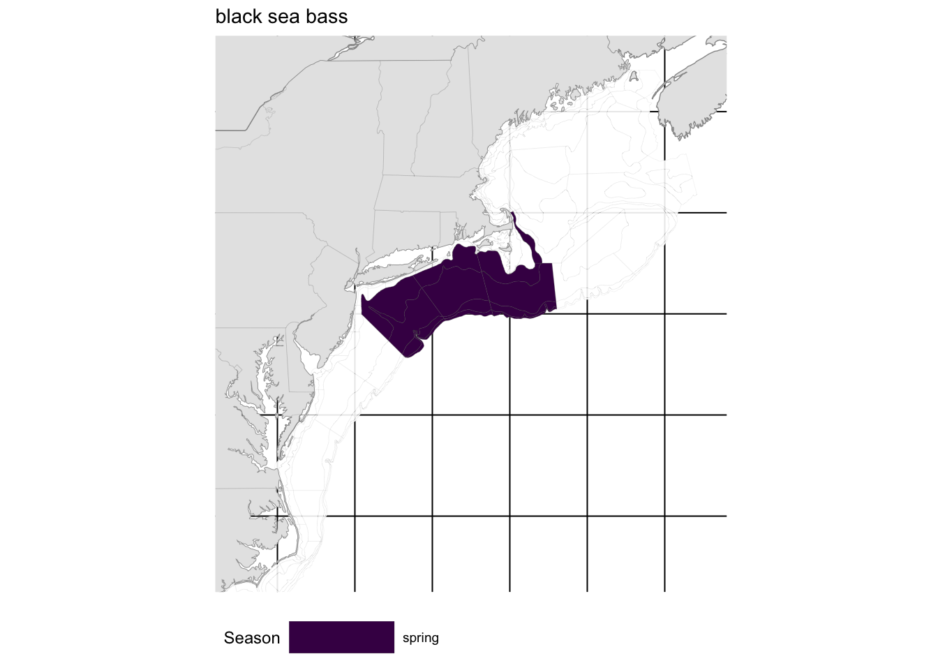
Figure 1.1: Strata map for the northern component of the black sea bass (Centropristis striata) stock on the NE shelf.

A note on figures

Unless otherwise noted, time series in this document are represented by dark blue lines. Estimates of linear trends and regime shifts are included on plots when found to be significant (p < 0.05), and are shown by light blue and green lines respectively. Trend strengths and confidence intervals are also included in plot titles when trends are present. Trends were modeled using a GLS model selection approach (see Hardison et al. 2019 for details).

Last updated on July 26 2019.

2 Temperature

An optimal interpolation procedure was used to estimate NE Shelf surface and bottom temperatures for two seasonal time frames (see methods). The temperature estimates were standardized to April 3 and October 11 for spring and fall over the period 1968-2018. Surface and bottom temperature within the northern component of the black sea bass stock area are shown below.

Bottom Temperature

Thermal conditions on the Northeast Shelf have changed in recent decades. Within the geographic area occupied by the northern component of the black sea bass stock, the spring bottom temperatures have been variable but without clear trend. However, it is important to note that bottom ocean temperature in the fall throughout the Middle Atlantic Bight has significantly warmed by about 2.1 °C (Kleisner et al. (2017)). Between the periods 1968-1978 and 2001-2012 in the spring, the center of biomass of black sea bass in the Middle Atlantic Bight has significantly shifted to the northeast (Kleisner et al. (2016)), likely tracking the local climate velocity of the region throughout the entire year given that no significant trend is observed in bottom ocean temperature in the spring. Laboratory studies of adult black sea bass physiology suggests that maximum metabolic performance occurs at a water temperature of 24.4 oC with decreased performance at warmer temperatures (Slesinger et al. (2019)). Ocean temperature in the U.S. NES is projected to increase above 24°C over the next 80-years in the southern portion of the northern stock’s range (Saba et al. (2016)). Therefore, it is likely black sea bass range will continue to shift poleward as the ocean continues to warm.

Surface Temperature

Similar to spring bottom temperature, spring surface temperature within the geographic area occupied by the northern component of the black sea bass stock has not changed significantly over time, however there was an anomalously low period around 1980.

3 Salinity

An optimal interpolation procedure was used to estimate NE Shelf surface and bottom salinity for two seasonal time frames (see methods). Though collected with temperature data, reliable instrumentation limits this time series to 1992-2018. The salinity estimates were standardized to April 3 and October 11 for spring and fall. Spring surface and bottom salinities within the northern component of the black sea bass stock area are shown below.

Bottom Salinity

Spring bottom salinity has increased over time within the northern component of the black sea bass stock stock area, with a change point increase in salinity in 2000.

Surface Salinity

Spring surface salinity has increased over time within the northern component of the black sea bass stock stock area, with a change point increase in salinity in 2013.

4 Chlorophyll

The concentration of chlorophyll was measured with a suite of satellite sensors and merged into a single dataset (see methods). Spring chlorophyll concentrations in the northern component of the black sea bass stock area are shown below.

Chlorophyll concentration in the stock area

Spring chlorophyll concentration has varied episodically but without trend over time within the northern component of the black sea bass stock stock area.

5 Zooplankton

There is little information on the diet of black sea bass larvae, though it is likely they feed on copepods and other zooplankton (TUCKER Jr (1989)).

Copepod abundance

The most abundant copepod species in this region are Calanus finmarchicus, Centropages typicus, and Pseudocalanus spp. While there is significant interannual variability in the abundance of these species, no clear trends have been observed over multiple decades.

Non-copepod zooplankton abundance

The most abundant non-copepod zooplankton species in this region are Appendicularians, Chaetognatha, and Gastropoda. While there is significant interannual variability in the abundance of these species, no clear trends have been observed over multiple decades.

6 Habitat and abundance

Occurrence probability

The probability of occurrence was estimated using random forest classification models (see methods). The mean annual probabilities were extracted for the spring stock definition area. These data provide an estimate of the potential use of the habitat associated with the northern component of the black sea bass stock definition.

Habitat area

The area of the Northeast Shelf with an estimated occurrence probability of 0.25 for the northern component of the black sea bass stock was determined for the stock area and the ecosystem.

Ecosystem area

7 Methods

Surface and Bottom Temperature and Salinity

7.0.1 Study System

The U.S. Northeast Shelf ecosystem, which roughly aligns with the boundaries of the Northeast U.S. Continental Shelf Large Marine Ecosystem (LME), is the study area for the surface and bottom thermal environments. Surface and bottom temperatures were estimated over a 0.1° latitude/longitude grid, termed the estimation grid, which circumscribes the range of ecosystem assessment areas in the region. The difference between the extents of the estimation grid from the extent of the LME relate to the resource management programs that are the sources of the data, which are focused on fishery management needs in the region.

7.0.2 Data Source

Temperature and salinity were collected on the Northeast Shelf as part of ongoing resource and ecosystem surveys conducted by the Northeast Fisheries Science Center. Water column temperatures have been collected contemporaneously to trawl tows associated with a bottom trawl survey beginning in the fall of 1963 and five years later during spring (Despres-Patanjo, Azarovitz, and Byrne 1988). In addition, the ecosystem has been surveyed by multiple sampling programs with varying sampling designs. The two most comprehensive monitoring programs over the study period were the MARMAP (1977-1987) and the Ecosystem Monitoring Program or EcoMon (1992-present) programs, both serving as shelf-wide surveys of the ecosystem (Sherman et al. 1998; J. Kane 2007). Temperature measurements were made with a mix of Conductivity Temperature and Depth (CTD) instruments, analog XBT, digital XBT, mechanical BT, glass thermometers (bottle temps) and trawl mounted temperature loggers instruments collecting either water column profiles or temperatures measured at targeted depths. Salinity measurements used in this analysis was limited to 1992-2017 when CTD instrument were used. Surface and bottom temperatures were identified from these measurements. Temperatures representing the spring period include data collected during the months of February to June; however, 99% of the samples were collected during the months of March to May. Likewise, the fall period samples include data collected during September to December, with 99% of the samples collected during September to November. The total number of surface temperature measurements were 14,540 and 14,666 for spring and fall, respectively; and, 14,450 and 14,656 for spring and fall bottom temperature, respectively. On average, there were 290 temperature measurements by season, depth, and year. The number of salinity observation per year were similar.

7.0.3 Interpolation Procedure

Seasonal surface and bottom temperature fields were estimated using an optimal interpolation approach. The optimal interpolation combined a climatological depiction of temperature and an annual estimates based on the data for a particular depth and season. (There were a number of precursor steps that are described below.). The surveys used to collect the data were conducted during the same period each year, however, there was variation in survey timing. To account for this, temperatures were standardized to a collection date of April 3 for spring surveys and October 11 for fall using linear regression for each depth and season over the sample grid (see Appendix, Figure A1). For each depth and season, annual shelf-wide mean temperatures were calculated using the data from sample grid locations with at least 80% of the time series present. The annual observations were then transformed to anomalies by subtracting the appropriate annual mean. All anomalies for a season and depth were combined over years into a single anomaly field or climatology.

The annual estimate of temperature for a depth and season was imputed by used universal kriging to estimate the temperature over the estimation grid with depth as a covariate. The kriging yielded temperature estimates and a variance estimate over the same grid. The optimal interpolation field was assembled by combining the annual estimate and information from the anomaly climatology. The climatology was re-leveled from anomaly values to temperatures by adding back the appropriate annual mean. For each location in the estimation grid, temperature was calculated as a weighted mean between the kriged annual estimate and the releveled climatology. The weightings in the calculations were partitioned based on the variance field of the annual kriging. The field was divided into quartiles from low to high variance with the weighting ratio of annual:climatology temperatures of 4:1, 3:1, 2:1, and 1:1, respectively. Hence, in areas of low variance the weighted mean was based on a weighting of 4:1, which would reflect a higher contribution of information from the annual estimate and thus be closer to an observation. In areas with high variance, the weighting ratio of 1:1 would reflect a greater effect of the climatology in determining the interpolation estimate.

The optimal interpolation temperature fields were evaluated using cross validation and a comparison to external data. The performance of optimal interpolation was compared to the predictive skill of using either the climatology or annual interpolation alone by doing ten random cross validations of each treatment. Each random draw of training and test sets sampled 3% of the data for the test set, or about 500 observations per draw. The temperature fields were fit with the training data and compared with the test set data. The lowest error rates were realized with the optimal interpolation contrasted with highest predictive error associated with fields based on the climatology alone (see Appendix, Figure A2). The spatial distribution of error had distinct depth and seasonal patterns. The spatial errors associated with the surface estimates were generally low with the exception of a few locations along the shelf break between latitudes 39-41°N; the spatial error in the bottom temperature varied by season, and was concentrated along the shelf break in spring and across the shelf between latitudes 36-40°N in fall (see Appendix, Figure A3). The optimal interpolation data were also compared to external data from other collection programs. The absolute errors between surface temperature data collected by satellites and the interpolation had interquartile ranges of approximately ±0.75°C (see Appendix, Figure A4). The absolute error in a comparison of interpolated bottom temperature to opportunist sampling was approximately ±0.75°C for spring bottom temperature and approximately 0.75-1.0°C in the fall. Salinity was estimated in the same way with the exception of collection correction, which was deemed unnecessary for the salinity data.

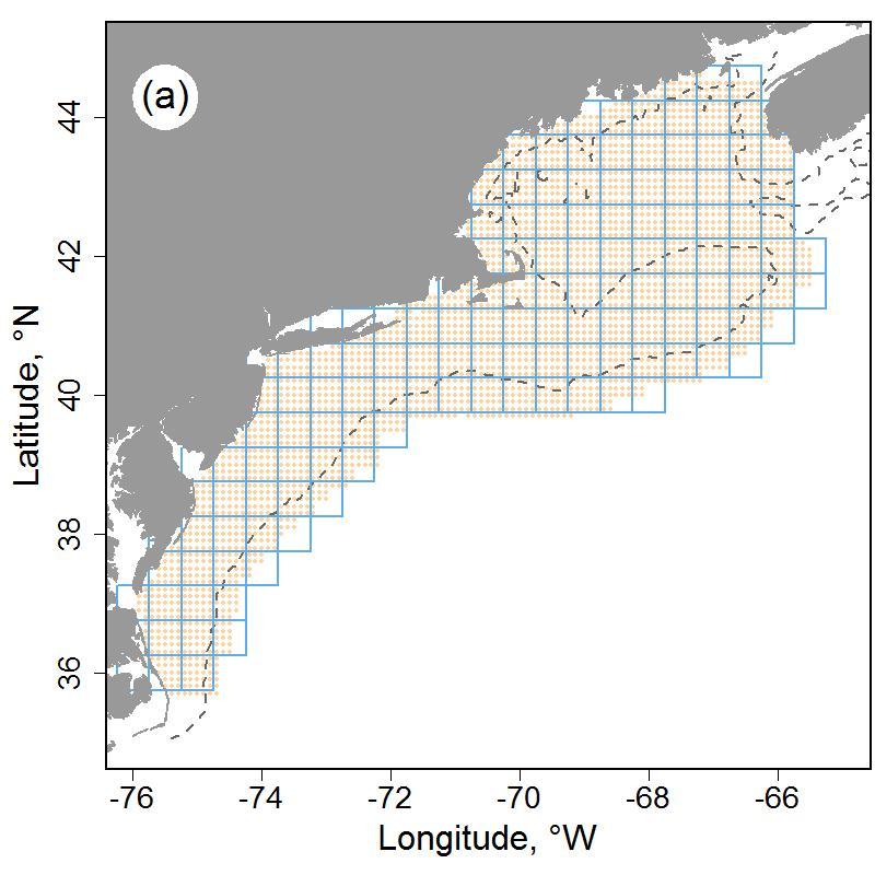
Figure 7.1: Map of the study system with half-degree sample grid (blue lines) and extent of estimation grid shown in beige points (a). Major features of the study system with shelf break marked in purple line (b). 100m depth shown as dashed line.

Chlorophyll data

Chlorophyll a concentration ([Chl]) data extracted from satellite remote-sensing databases based on measurements made with the Sea-viewing Wide Field of View Sensor (SeaWiFS), Moderate Resolution Imaging Spectroradiometer on the Aqua satellite (MODIS), Medium Resolution Imaging Spectrometer (MERIS), and Visible and Infrared Imaging/Radiometer Suite (VIIRS) sensors. We used the Garver, Siegel, Maritorena Model (GSM) merged data product at 100 km (equivalent to a 1° grid) and 8-day spatial and temporal resolutions, respectively, obtained from the Hermes GlobColour website. These four sensors provide an overlapping time series of [Chl] during the period 1997 to 2018 and were combined based on a bio-optical model inversion algorithm (Maritorena et al. 2010).

Zooplankton abundance

Zooplankton abundance is measured by the Ecosystem Monitoring Program (EcoMon), which conducts shelf-wide bimonthly surveys of the NES ecosystem (J. Kane 2007). Zooplankton and ichthyoplankton are collected throughout the water column to a maximum depth of 200 m using paired 61-cm Bongo samplers equipped with 333-micron mesh nets. Sample location in this survey is based on a randomized strata design, with strata defined by bathymetry and along-shelf location. Plankton taxa are sorted and identified. We used the bio-volume of the 18 most abundant taxonomic categories as potential predictor variables (Table 2). The zooplankton sample time series has some missing values, which necessitated the removal of spring data for the years 1989, 1990, 1991, and 1994 and fall data for the years 1989, 1990, and 1992. The data for each seasonal time frame was interpolated to a complete field over the estimation grid using ordinary kriging.

7.0.4

Table 7.1: Variable and species names for the 18 most abundant zooplankton taxa in EcoMon survey data.

Variable name	Taxa
acarspp	Acartia spp.
calfin	Calanus finmarchicus
chaeto	Chaetognatha
cham	Centropages hamatus
cirr	Cirripedia
ctyp	Centropages typicus
echino	Echinodermata
evadnespp	Evadne spp.
gas	Gastropoda
hyper	Hyperiidea
larvaceans	Appendicularians
mlucens	Metridia lucens
oithspp	Oithona spp.
para	Paracalanus parvus
penilia	Penilia spp.
pseudo	Pseudocalanus spp.
salps	Salpa
tlong	Temora longicornis

Occupancy models

Occupancy and productivity habitats for Atlantic menhaden were estimated with random forest classification and regression models using a suite of static and dynamic predictor variables. Variation in species presence or absence and biomass across space, bathymetry factors, productivity factors, and climate factors were tested. Models were constructed separately for spring and fall seasons. The response variables were the occurrence and catch-per-unit-effort of Atlantic menhaden in the Northeast Fisheries Science Center bottom trawl survey, which is a fishery-independent survey on the Northeast US Shelf. The survey is conducted in the spring and fall of the year and is based on a stratified random design, which provides both spatial and temporal depictions of fish and macroinvertebrate abundances (Grosslein 1969). The independent or predictor variable set included physical environment variables, habitat descriptors, zooplankton variables, and remote sensing variables; the variables will be described in more detail below. Occupancy models were fit as two-factor classification models (absence as 0; presence as 1) using the randomForest R package (Liaw and Wiener 2002).

Prior to fitting the model, the independent variable set was first tested for multi-collinearity among the predictors and correlated variables were eliminated (R package Evans and Murphy (2018), version 2.1-3). From this reduced set of predictors, the final model variables were selected utilizing the model selection criteria of (Murphy, Evans, and Storfer 2010) as implemented in rfUtilities. Productivity models were fit as regression models with log10 transformed biomass-per-unit-effort as the response variable and the same starting set of predictor variables as in the occupancy models. As with the occupancy models, independent variables were tested for multi-collinearity and the model selection criteria was applied. Habitat was estimated from the model fits over a standard 0.1° grid, which circumscribes the range of ecosystem assessment areas in the region.

Three types of visualizations were created from the output of the tree models. The first visualization was used to see the average probability of occupancy over space and the rate of change (Sen’s slope) in occupancy over the years. The second visualization was used to see the mean occupancy gradient magnitude, or frontal strength and the rate of change (Sen’s slope) in occupancy gradient magnitude over the years. Gradient magnitude was calculated by calculating the median of the occupancy probabilities with a moving window and then summing those medians with a moving window with a matrix of weights. The third visualization was used to see the average biomass over space and the rate of change (Sen’s slope) in biomass over the years. Trends in total occupancy habitat area, with occupancy probabilities of 25, 50, and 75% over time were plotted as well by calculating the sum of the area with occupancy probabilities at each percentage during each year.

Following from the 2018 ECSA for summer flounder, the methodology was changed by the conversion of salinity, surface and bottom, from a dynamic variable to a static variable. By so doing, the fitting period is extended from 1992-2017 to 1976-2018. Dynamic salinity data was limited by the time series of modern instrumentation, which began in 1992. In the 2018 model fits, dynamic salinity was not an important variable in any species model; hence, conversion to a static variable was of little consequence.

7.0.5 Minimum swept area abundance based on habitat informed dynamic re-stratification

Estimates of the numbers and biomass minimum population size of stocks was determined by re-stratifying the habitat each year depending on the distribution of occupancy habitat. The habitat area was restricted to the portion of the shelf associated with the stock based on the roster of bottom trawl strata consider to comprise the stock area. To raise an annual estimate, the habitat was partitioned into ten intervals based on the probability of occurrence from the species distribution model. The partitions were based on equal intervals of occurrence probability; hence, the size of each habitat strata could vary. The trawl catch per unit effort values were assigned to the appropriate habitat strata based on the habitat score where the trawl was made. Once the requisite trawl hauls associated with a habitat strata were identified, a mean catch per unit effort was determined and raised to a total minimum population estimate for that stratum assuming a constant trawl path area of 0.024 km ². The total population was the sum of the estimates for the ten strata.

\(Total\;numbers\;or\;biomass =\sum_{i=1}^{10} (strata\;area/trawl\;path\;area) * mean\;CPUE\)

These estimates were conditioned on three options intended to ameliorate some of the issues associated with the variability in survey catch rates. The first allowed for the application of catch per unit effort data from either the stock area only or including tows from outside the stock area if they were collected in areas with habitat scores matching the probability from the intervals in the stock area. It was felt this may enhance the estimate by increasing the sample size for key strata. The second option provided the choice of performing a test for outliers on the trawl catch per unit effort data. The boxplot command in R was used to identify the outliers for removal. The last option involved whether to apply a smoothing across the mean catch per unit effort estimates in each strata. If the option was invoked, a loess smoother (span = 0.75) was applied to generate the smoothed catch rates; the procedure also had the benefit of interpolating and extrapolating a rate to a habitat strata that may not have had catch samples associated with it. Therefore, for each species/stock, an estimate of seasonal total abundance or biomass minimum population size will have eight realizations that test the sensitively of the calculations to these three formulation choices.

7.0.6 Predictor Variables

Static variables were kept constant over years where dynamic variables varied annually. Hence, the length of the time series of model fits is constrained by the shortest dynamic variable time series to meet the requirement of complete cases in the Random Forest fitting. The fitting time series was constrained to 1992 – 2016, which was determined by the length of the station salinity data.

7.0.7 Physical environment

Station data included observations made contemporaneously to survey bottom trawl stations. Depth of the station was used as a static variable in the analysis. The observed depth was used in model fitting where model predictions were based on depths from the ETOPO1 dataset, which provided Northeast Shelf bathymetry at a resolution of 0.0167° (below).

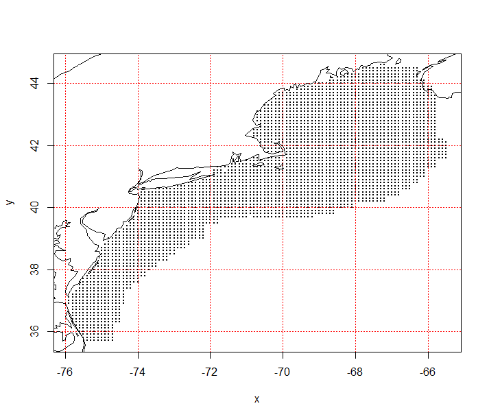
Figure 7.2: Estimation grid for predictor variable and habitat estimates, grid location spaced by 0.1° longitude and latitude.

Surface and bottom water temperature and salinity were used as dynamic variables in the analysis. Temperature and salinity on the NE Shelf was collected using Conductivity/Temperature/Depth (CTD) instruments with the most complete sample coverage associated with spring (February –April) and fall (September-November) time frames. Surface and bottom temperatures were used to develop date of collection corrections using linear regression for each time frame. Temperatures were standardized to a collection date of April 3 for spring collections and October 11 for fall. A date of collection correction was not indicated for salinity data. The observed date-corrected temperature (°C) and uncorrected salinity data (PSU) was used in model fitting.

Model predictions were based on temperature and salinity fields using an optimal interpolation approach where annual data were combined with a climatology by season. For a half degree grid of the ecosystem, mean bottom temperature or salinity was calculated by year and season. For grid locations that had data for at least 80% of the time series, the data from those locals were used to calculate a seasonal mean. The annual seasonal means were used to calculate anomalies, which were combined over the time series to provide seasonal, surface and bottom anomaly climatologies.

Returning to the raw data, the observations for a year, season, and depth were then used to estimate an annual field using universal kriging with depth as a covariate. The kriging was done on a standard 0.1° grid using the automap (Hiemstra et al. 2008, version 1.0–14). The annual field was then combined with the climatology anomaly field, adjusted by the annual mean, using the variance field from the kriging as the basis for a weighted mean between the two. The variance field was divided into quartiles with the first quartile (lowest kriging variance) carrying a weighting of 4:1 between the annual and climatology values. Hence, the optimal interpolated field at these locations were skewed towards the annual data reflecting their proximity to actual data locations and low kriging variance associated with them. The weighting ratio shifted to 1:1 in the highest variance quartile reflecting less information from the annual field and more from the climatology.

7.0.8 Habitat Descriptors

Habitat descriptors are a series of static variables that reflect the shape and complexity of benthic habitats. Since the response variables for these models are derived from bottom trawl gear, naturally the range of candidate taxa for modelling is skewed to benthic organisms, making these descriptors particularly relevant. Most of the variables are based on depth measurement, including the complexity, BBI, VRM, Prcurv, rugostity, seabedforms, slp, and slpslp variables (Table 1). The soft-sed variable is based on benthic sediment grain size and the vorticity variable is based on current estimates.

7.0.9 Zooplankton Data

Zooplankton abundance is measured by the Ecosystem Monitoring Program (EcoMon), which conducts shelf-wide bimonthly surveys of the NES ecosystem (J. Kane 2007). Zooplankton and ichthyoplankton are collected throughout the water column to a maximum depth of 200 m using paired 61-cm Bongo samplers equipped with 333-micron mesh nets. Sample location in this survey is based on a randomized strata design, with strata defined by bathymetry and along-shelf location. Plankton taxa are sorted and identified. We used the bio-volume of the 18 most abundant taxonomic categories as potential predictor variables (Table 2). The zooplankton sample time series has some missing values which were ameliorated by summing data over five-year time steps for each seasonal time frame and interpolating a complete field using ordinary kriging. Thus, for example, the data for spring 2000 would include the available data from 1998-2002 tows.

7.0.10 Remote Sensing Data

Chlorophyll concentration and SST from remote sensing sources were applied in the habitat models as static variables. Chlorophyll and SST were summarized as monthly means with their associated gradient magnitude or frontal fields. The basis for the chlorophyll concentration was measurements made with the Sea-viewing Wide Field of View Sensor (SeaWiFS), Moderate Resolution Imaging Spectroradiometer on the Aqua satellite (MODIS), Medium Resolution Imaging Spectrometer (MERIS), and Visible and Infrared Imaging/Radiometer Suite (VIIRS) sensors during the period 1997-2016. The data is a merged product using the Garver, Siegel, Maritorena Model (GSM) algorithm obtained from the Hermes GlobColour website.

These four sensors provide an overlapping time series of chlorophyll concentration during the period and were combined based on a bio-optical model inversion algorithm (Maritorena et al. 2010). Monthly SST fields were based on data from the MODIS Terra sensor data available from the Ocean Color Website. From these data, mean monthly fields were generated for both chlorophyll and SST. There are a range of methods used to identify fronts (Belkin and O’Reilly 2009) in oceanographic data that usually apply some focal filter to reduce noise and identify gradient magnitude with a Sobel filter. These calculations were done in R using the raster package (Hijmans 2017, version 2.6–7) using a 3 by 3 mean focal filter and a Sobel filter to generate x and y derivatives, which are then used to calculate gradient magnitude.

7.0.11 Model Selection Criteria and Variable Importance

The habitat models were evaluated for fit based on out-of-bag classification accuracy. For occupancy models accuracy, AUC (Area Under the ROC Curve), and Cohen’s Kappa were calculated using the irr R package (Gamer et al. 2012, version 0.84). For regression models, the variance explained by the model, mean absolute error, the root mean square error, and bias were calculated using the Metrics R package (Hamner and Frasco 2018, version 0.1.3). To evaluate variable importance in both occupancy and regression models, we plotted the number of times a variable was the root variable versus the mean minimum node depth for the variable, highlighting the top ten important variables using the randomForestExplainer R package (Paluszynska and Biecek 2017, version 0.9). For occupancy models we also plotted the Gini index decrease versus accuracy decrease, whereas for the regression models we plotted node purity increase versus MSE increase, also highlighting the top ten most important variables.

7.0.12

Table 7.2: Habitat descriptors used in occupancy model parameterization.

Variables	Notes	References
Complexity - Terrain Ruggedness Index	The difference in elevation values from a center cell and the eight cells immediately surrounding it. Each of the difference values are squared to make them all positive and averaged. The index is the square root of this average.	Riley, DeGloria, and Elliot (1999)
Namera bpi	BPI is a second order derivative of the surface depth using the TNC Northwest Atlantic Marine Ecoregional Assessment (“NAMERA”) data with an inner radius=5 and outer radius=50.	Lundblad et al. (2006)
Namera_vrm	Vector Ruggedness Measure (VRM) measures terrain ruggedness as the variation in three-dimensional orientation of grid cells within a neighborhood based the TNC Northwest Atlantic Marine Ecoregional Assessment (“NAMERA”) data.	Hobson (1972); Sappington, Longshore, and Thompson (2007)
Prcurv (2 km, 10 km, and 20 km)	Benthic profile curvature at 2km, 10km and 20 km spatial scales was derived from depth data.	A. Winship et al. (2018)
Rugosity	A measure of small-scale variations of amplitude in the height of a surface, the ratio of the real to the geometric surface area.	Friedman et al. (2012)
seabedforms	Seabed topography as measured by a combination of seabed position and slope.	www.northeastoceandata.org
Slp (2 km, 10 km, and 20 km)	Benthic slope at 2km, 10km and 20km spatial scales.	A. Winship et al. (2018)
Slpslp (2 km, 10 km, and 20 km)	Benthic slope of slope at 2km, 10km and 20km spatial scales	A. Winship et al. (2018)
soft_sed	Soft-sediments is based on grain size distribution from the USGS usSeabed: Atlantic coast offshore surficial sediment data.	www.northeastoceandata.org
Vort (fall - fa; spring - sp; summer - su; winter - wi)	Benthic current vorticity at a 1/6 degree (approx. 19 km) spatial scale.	Kinlan et al. (2016)

Diet composition

NEFSC bottom-trawl sampling occurs twice annually in the spring (March-May) and fall (September-November). The survey area encompasses about 293,000 square km of continental shelf from Cape Hatteras, NC, to Nova Scotia, Canada in depths from 8-400 m. Food habits sampling has been conducted since 1973.

Stomachs are collected at sea by NEFSC, and have been primarily analyzed at sea since 1981. Total stomach volume is estimated, each prey item is identified and sorted to the lowest possible taxonomic level, and the proportion of each prey item is estimated. Detailed methods are described in Link and Almeida (2000). Prey composition percent by weight was calculated using a weighted mean (\(\overline{W_{ijs}}\)) (Link and Almeida 2000; Smith and Link 2010) to estimate mean weight of prey \(i\) in predator \(j\) for statistical group \(s\). Note: Prey volumes are used as proxies for prey weight. It may be calculated as

\[ \overline{W_{ijs}} = \frac{\sum_{t=1}^{N_{ts}}N_{jts}\overline{w_{ijts}}}{N_{ts}} \]

where \(t\) represents an individual bottom trawl tow, \(N_{jts}\) is the number of predator \(j\) stomachs in tow \(t\) for statistical group \(s\), \(N_{ts}\) is the number of tows in statistical group \(s\), and

\[ \overline{w_{ijts}} = \frac{\sum_{k=1}^{N_{jts}}w_{ijtsk}}{N_{jts}} \]

Appendix

7.0.13 Date of collection correction

The dates of survey data collection varied by year. To date correct temperature measurements, regressions were estimated between temperature and day of the year over the sample grid (0.5° grid) by season and depth. Spring data were transformed to a temperature representing April 3 and fall to October 11 based on the slope estimates shown in the maps in Figure A1.

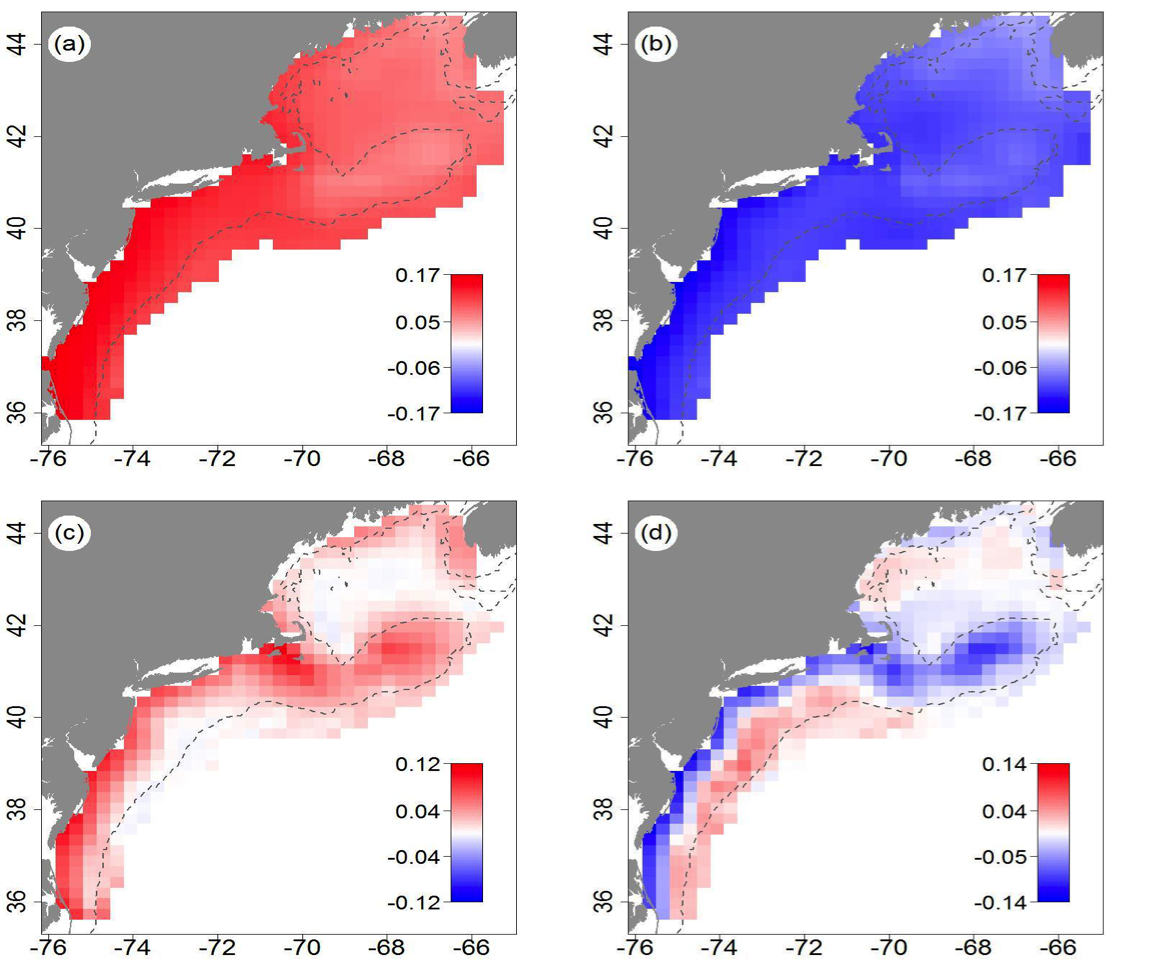
Figure 7.3: Spring (a) and fall (b) linear slope coefficients used to date correct surface temperature to standard spring and fall dates; same for spring (c) and fall (d) bottom temperature correction.

7.0.14 Cross validation performance of temperature interpolation

A series of random draws of training and test sets were taken to evaluate the predictive skill of the estimation procedure. A set of climatology, annual interpolation, or optimal interpolation fields were estimated using the training set and compared to the held-out test set.

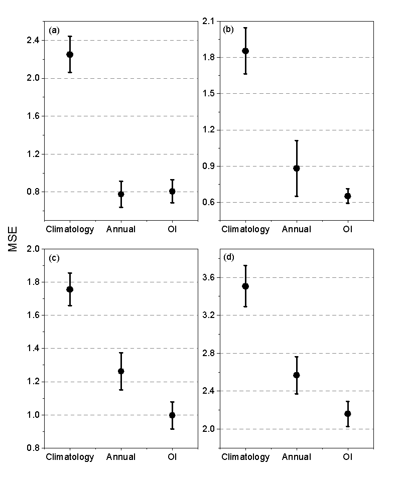
Figure 7.4: Mean and 95% confidence intervals of squared errors for spring (a) and fall (b) surface temperature estimates based on climatology, annual interpolation, and optimal interpolation (OI); same data for spring (c) and fall (d) bottom temperature estimates.

The distribution of errors from the optimal interpolation test sets were evaluated spatially to determine where the larger errors occurred and what ecosystem features they are associated with.

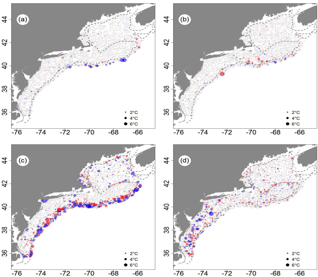
Figure 7.5: Mean absolute error by 0.1 degree latitude and longitude intervals for spring (a) and fall (b) surface temperature; same data for spring (c) and fall (d) bottom temperature. Red indicates a positive error where blue indicates negative.

7.0.15 Comparisons to external data sources

Sea surface temperature estimated in this study were compared to the OISST dataset serving as a source of data for external comparison. The OISST data for April 3 (spring) and October 11 (fall) over the period 1982-2017 were extracted on the same 0.5° grid used in the study. Time series of matching spring and fall temperatures were differenced (external minus interpolation data) and presented in the figure below (sample size for surface spring and fall data were 5220 and 5365, respectively). The interquartile range for the surface comparisons were generally symmetric around zero with differences between 0.5-1°C. Bottom temperature estimated in this study were compared to the data from a cooperative data collection program for external comparison. The “Environmental Monitors on Lobster Traps” (EMOLT) is a cooperative research program that collects bottom temperatures. The data for spring and fall were extracted from rasters of the study data to match the extremal data. The external data covered the period 1968-2017, with 360 data points for the spring and 728 for the fall. Spring bottom comparisons yielded the smallest interquartile range of differences less than 0.5°C, where fall comparisons were slightly larger and biased to lower interpolation estimates compared to the external data.

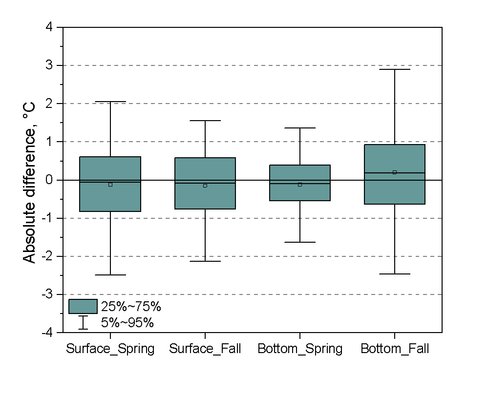
Figure 7.6: Box plots (box: interquartile range, whisker: 5-95% range, square symbol: mean, line: median) of the difference between external and interpolation data.

8 Document automation

To facilitate speedy document creation many steps have been automated. Species specific information are passed as arguments to a default rmarkdown template (the backbone of this document). This template is then rendered into a book using the package bookdown. Prior to rendering the data are pre-processed and output as .RData files for use in the automation steps. The specific steps are as follows:

Manunal preprocessing

1. model outputs are created in the form of annual raster files (.RData) for chlorophyll, zooplankton, temperature, salinity, ocurrance probability (species specific), and biomass (species specific).
2. These sets of annual raster files are collapsed into a single stack (.RData) using the script collapse_to_stack.R. The resulting stacked raster files are exported with this package.

Automation

1. create_template.R is run to create the species specific .Rmd document with the following arguments (for additional arguments, refer to ?create_template). For {{COMMON_NAME}}:

create_template(stock_name = {{STOCK_NAME}}, render_book=TRUE, output_dir = here::here("docs"))

2. The species specific Rmd file is then rendered. During this step:

• The stacked raster files are clipped to the appropriate seasonal stock area (See Figure 1.1 ) using stars_to_series.R.

• A linear trend is fitted (using the package ecotrend) to the environmental variables (temperature and salinity), chlorophyll, and species biomass. The resulting fit is ONLY plotted if found to be significant at the 5% level.

• A regime mean is also fit (using STARS_v18.R) and displayed on all plots.

• Zooplankton:

• Occupancy probability:

3. This document (the one you are viewing) will then automatically open in a web browser and all associated files can be found in the docs\{{STOCK_NAME}} folder in your current working directory.
4. These steps are repeated for additional species.

References

Belkin, Igor M, and John E O’Reilly. 2009. “An Algorithm for Oceanic Front Detection in Chlorophyll and Sst Satellite Imagery.” Journal of Marine Systems 78 (3). Elsevier: 319–26.

Despres-Patanjo, Linda I, Thomas R Azarovitz, and Charles J Byrne. 1988. “Twenty-Five Years of Fish Surveys in the Northwest Atlantic: The Nmfs Northeast Fisheries Center’s Bottom Trawl Survey Program.” Marine Fisheries Review 50 (4). NMFS, Scientific Publications Office: 69–71.

Evans, Jeffrey S., and Melanie A. Murphy. 2018. RfUtilities. https://cran.r-project.org/package=rfUtilities.

Friedman, Ariell, Oscar Pizarro, Stefan B. Williams, and Matthew Johnson-Roberson. 2012. “Multi-Scale Measures of Rugosity, Slope and Aspect from Benthic Stereo Image Reconstructions.” PLoS ONE 7 (12). doi:10.1371/journal.pone.0050440.

Gamer, Matthias, Jim Lemon, Ian Fellows, and Puspendra Singh. 2012. Irr: Various Coefficients of Interrater Reliability and Agreement. https://CRAN.R-project.org/package=irr.

Grosslein, MD. 1969. Groundfish Survey Methods. Bureau of Commercial Fisheries, Biological Laboratory. https://nefsc.noaa.gov/publications/series/whlrd/whlrd6902.pdf.

Hamner, Ben, and Michael Frasco. 2018. Metrics: Evaluation Metrics for Machine Learning. https://CRAN.R-project.org/package=Metrics.

Hardison, Sean, Charles T Perretti, Geret S DePiper, and Andrew Beet. 2019. “A Simulation Study of Trend Detection Methods for Integrated Ecosystem Assessment.” ICES Journal of Marine Science.

Hiemstra, P.H., E.J. Pebesma, C.J.W. Twenh"ofel, and G.B.M. Heuvelink. 2008. “Real-time automatic interpolation of ambient gamma dose rates from the Dutch Radioactivity Monitoring Network.” Computers & Geosciences.

Hijmans, Robert J. 2017. Raster: Geographic Data Analysis and Modeling. https://CRAN.R-project.org/package=raster.

Kane, Joseph. 2007. “Zooplankton abundance trends on Georges Bank, 1977-2004.” ICES Journal of Marine Science 64 (5): 909–19. doi:10.1093/icesjms/fsm066.

Kinlan, Brian P., Arliss J. Winship, Timothy P. White, and John Christensen. 2016. “Modeling At-Sea Occurrence and Abundance of Marine Birds to Support Atlantic Marine Renewable Energy Planning Phase I Report.”

Kleisner, Kristin M, Michael J Fogarty, Sally McGee, Analie Barnett, Paula Fratantoni, Jennifer Greene, Jonathan A Hare, et al. 2016. “The Effects of Sub-Regional Climate Velocity on the Distribution and Spatial Extent of Marine Species Assemblages.” PloS One 11 (2). Public Library of Science: e0149220.

Kleisner, Kristin M, Michael J Fogarty, Sally McGee, Jonathan A Hare, Skye Moret, Charles T Perretti, and Vincent S Saba. 2017. “Marine Species Distribution Shifts on the Us Northeast Continental Shelf Under Continued Ocean Warming.” Progress in Oceanography 153. Elsevier: 24–36.

Liaw, Andy, and Matthew Wiener. 2002. “Classification and Regression by randomForest.” R News 2 (3): 18–22. https://CRAN.R-project.org/doc/Rnews/.

Link, Jason S., and Frank P. Almeida. 2000. An Overview and History of the Food Web Dynamics Program of the Northeast Fisheries Science Center. NOAA Technical Memorandum NMFS-NE-159. Woods Hole, MA. http://www.nefsc.noaa.gov/publications/tm/tm159/.

Lundblad, Emily R., Dawn J. Wright, Joyce Miller, Emily M. Larkin, Ronald Rinehart, David F. Naar, Brian T. Donahue, S. Miles Anderson, and Tim Battista. 2006. “A benthic terrain classification scheme for American Samoa.” Marine Geodesy 29 (2): 89–111. doi:10.1080/01490410600738021.

Murphy, Melanie A., Jeffrey S. Evans, and Andrew Storfer. 2010. “Quantifying Bufo boreas connectivity in Yellowstone National Park with landscape genetics.” Ecology 91 (1): 252–61. doi:10.1890/08-0879.1.

Paluszynska, Aleksandra, and Przemyslaw Biecek. 2017. randomForestExplainer: Explaining and Visualizing Random Forests in Terms of Variable Importance. https://CRAN.R-project.org/package=randomForestExplainer.

Riley, Shawn J, Stephen D DeGloria, and Robert Elliot. 1999. “A Terrain Ruggedness Index that Qauntifies Topographic Heterogeneity.” doi:citeulike-article-id:8858430.

Saba, Vincent S, Stephen M Griffies, Whit G Anderson, Michael Winton, Michael A Alexander, Thomas L Delworth, Jonathan A Hare, et al. 2016. “Enhanced Warming of the N Orthwest a Tlantic O Cean Under Climate Change.” Journal of Geophysical Research: Oceans 121 (1). Wiley Online Library: 118–32.

Sappington, J. M., Kathleen M. Longshore, and Daniel B. Thompson. 2007. “Quantifying Landscape Ruggedness for Animal Habitat Analysis: A Case Study Using Bighorn Sheep in the Mojave Desert.” Journal of Wildlife Management 71 (5): 1419–26. doi:10.2193/2005-723.

Sherman, Kenneth, A Solow, J Jossi, and J Kane. 1998. “Biodiversity and Abundance of the Zooplankton of the Northeast Shelf Ecosystem.” ICES Journal of Marine Science 55 (4). Oxford University Press: 730–38.

Slesinger, Emily, Alyssa Andres, Rachael Young, Brad Seibel, Vincent Saba, Beth Phelan, John Rosendale, Daniel Wieczorek, and Grace Saba. 2019. “The Effect of Ocean Warming on Black Sea Bass (Centropristis Striata) Aerobic Scope and Hypoxia Tolerance.” PloS One 14 (6). Public Library of Science: e0218390.

Smith, Brian E., and Jason S. Link. 2010. The Trophic Dynamics of 50 Finfish and 2 Squid Species on the Northeast US Continental Shelf. NOAA Technichal Memorandum NMFS-NE-216. National Marine Fisheries Service, 166 Water Street, Woods Hole, MA 02543-1026. http://www.nefsc.noaa.gov/publications/tm/tm216/.

TUCKER Jr, JOHN W. 1989. “Energy Utilization in Lay Anchovy, Anchoa Mitchilli, and Black Sea Bass, Centropristis Striata Eggs and Larvae.” Fish. Bull., US 78: 279–193.

Winship, A.J., Kinlan B.P., T.P. White, and J.B. Leirness. 2018. “Modeling At-Sea Density of Marine Birds to Support Atlantic Marine Renewable Energy Planning: Final Report.” OCS Study BOEM 2018-010.